Introduction

GitHub repository · Runnable examples · Stochastic Minds
Source code: github.com/benovamurat/solow — stars, issues, and contributions welcome.
Solow is a complete statistical-modeling, econometrics, and data-visualization toolkit for Rust. It provides estimators for a wide range of statistical models, along with statistical tests, diagnostics, and data exploration — entirely in safe, dependency-light Rust.
If you have used the canonical Python statistics stack (NumPy / SciPy together with the standard econometrics-modeling package), Solow will feel familiar: the model names, the result quantities, and the formula syntax all mirror that ecosystem. The difference is that Solow is a from-scratch re-implementation in Rust, with no Python runtime and no system LAPACK/BLAS dependency.
Design principles
-
Pure Rust. The numerical core — linear algebra (SVD, eigendecomposition, Cholesky, QR, LU, pseudo-inverse), special functions (incomplete beta/gamma,
erf), and the statistical distributions — is implemented in pure Rust. The only foundational dependency isndarray. There is no system LAPACK/BLAS to install and no C toolchain to wrangle. -
Verified against a reference. Every numerical routine is cross-checked against an authoritative reference implementation of the same models. Golden fixtures are generated from that reference and committed to the repository; the test suite asserts agreement to a tight tolerance — most quantities to
1e-8, maximum-likelihood and variational-Bayes estimates to1e-6, and the formula engine to1e-12. This means a model you fit with Solow returns the same numbers you would get from the established tool, not merely numbers that "look right." -
Layered. Solow is a Cargo workspace of focused crates, each mirroring a module of a mature statistics library. You depend only on what you use, or pull in the umbrella
solowcrate to get everything behind one import. -
Faithful output. Results carry the same battery of inference statistics you expect: standard errors, t/z statistics, p-values, confidence intervals, information criteria, and (where applicable) robust covariances. A human-readable summary table renders the way you are used to seeing.
What is in the box
Solow covers, among other things:
| Area | Crate | Models / tools |
|---|---|---|
| Linear regression | solow-regression | OLS, WLS, GLS, quantile, rolling/recursive LS, robust covariances |
| Generalized linear models | solow-glm | Gaussian, Binomial, Poisson, Gamma, Inverse-Gaussian, Negative-Binomial, Tweedie |
| Discrete choice | solow-discrete | Logit, Probit, Poisson, MNLogit, Negative-Binomial, ordered, zero-inflated |
| Robust regression | solow-robust | M-estimation (Huber, Tukey biweight, Andrew wave) |
| Time series | solow-tsa | acf/pacf, ADF, KPSS, AutoReg, STL, Holt-Winters, Granger, cointegration |
| State space | solow-statespace | Kalman filter/smoother, SARIMAX, unobserved components, dynamic factor |
| Vector autoregression | solow-var | VAR, SVAR, VECM / Johansen |
| Survival / duration | solow-duration | Kaplan-Meier, Cox PH, log-rank |
| Multivariate | solow-multivariate | PCA, factor analysis, MANOVA, canonical correlation |
| Nonparametric | solow-nonparametric | LOWESS, kernel density, kernel regression |
| Statistical tests | solow-stats | normality, heteroskedasticity, autocorrelation, ANOVA, multiple testing |
| Distributions | solow-distributions | distributions and special functions (scipy-compatible) |
| Formula interface | solow-formula | patsy-style design matrices from a formula string |
| Summary tables | solow-summary | labeled results and fixed-width summary rendering |
| Python bindings | solow-py | import solow from Python (PyO3) |
See the Crate reference for the full workspace.
A taste
#![allow(unused)]
fn main() {
use ndarray::{array, Array1};
use solow_core::tools::{add_constant, HasConstant};
use solow_regression::LinearModel;

let x = array![[1.0], [2.0], [3.0], [4.0], [5.0]];
let y: Array1<f64> = array![1.1, 1.9, 3.2, 3.9, 5.1];

let design = add_constant(&x, true, HasConstant::Add).unwrap();
let res = LinearModel::ols(y, design).unwrap().fit().unwrap();

println!("R-squared = {:.3}", res.rsquared);
println!("coefficients = {:?}", res.params);
}
Read on to install Solow and work through a fuller quickstart.
Installation
Solow is a Cargo workspace of focused crates. You can depend on the single
crate you need, or on the umbrella solow crate that re-exports the whole
public API.
Requirements
- Rust 1.80 or newer (stable). Solow tracks the stable toolchain; the
repository pins it with a
rust-toolchain.toml. - No system math libraries. Solow's linear algebra and special functions are pure Rust, so there is no LAPACK, BLAS, or C compiler to install.
The only foundational third-party dependency is ndarray, which Solow uses
for its vector and matrix types (Array1<f64> / Array2<f64>).
Adding individual crates
Pick the crates that match what you are doing. For example, ordinary least squares plus the summary renderer:
[dependencies]
solow-core = "0.1"
solow-regression = "0.1"
solow-summary = "0.1"
ndarray = "0.16"
A few common combinations:
| Task | Crates |
|---|---|
| OLS / WLS / GLS | solow-core, solow-regression |
| GLM | solow-glm |
| Logit / Probit / Poisson | solow-discrete |
| Time-series tools and AutoReg | solow-tsa |
| SARIMAX / Kalman | solow-statespace |
| VAR / VECM | solow-var |
| Formula → design matrix | solow-formula |
| Rendered summary table | solow-summary |
Adding the umbrella crate
If you would rather have everything available behind one dependency, use the umbrella crate:
[dependencies]
solow = "0.1"
ndarray = "0.16"
Each library is then reachable as a module, and a prelude collects the most
common imports:
#![allow(unused)]
fn main() {
use solow::prelude::*;       // Array1, Array2, Axis, core error types
use solow::regression::LinearModel;
use solow::glm::{Family, Glm};
use solow::tsa::{acf, AutoReg, Trend};
}
Building from source
git clone https://github.com/solow-rs/solow
cd solow
cargo build --workspace
cargo test --workspace
Because the numerical core is pure Rust, this builds on Linux, macOS, and Windows with nothing more than a stable Rust toolchain.
Python users
Solow can also be imported from Python through the solow-py bindings (a native
CPython extension built with PyO3). That crate is its own standalone workspace.
See Using Solow from Python for the build steps and API.
Quickstart
This chapter fits an ordinary least squares (OLS) regression end to end: build a design matrix, estimate the model, read off the results, and render a summary table. It is the smallest complete example that touches the pieces you will use everywhere in Solow.
Set up the crate
[dependencies]
solow-core = "0.1"
solow-regression = "0.1"
solow-summary = "0.1"
ndarray = "0.16"
Fit an OLS model
Solow does not add an intercept for you (matching the convention of the
reference stack). You add the constant column explicitly with add_constant.
use ndarray::{array, Array1};
use solow_core::tools::{add_constant, HasConstant};
use solow_regression::LinearModel;

fn main() {
    // Predictor (one column) and response.
    let x = array![[1.0], [2.0], [3.0], [4.0], [5.0], [6.0]];
    let y: Array1<f64> = array![2.1, 3.9, 6.2, 7.8, 10.1, 12.0];

    // Prepend a constant column → design matrix with [const, x].
    let design = add_constant(&x, true, HasConstant::Add).unwrap();

    // Estimate by ordinary least squares.
    let res = LinearModel::ols(y, design).unwrap().fit().unwrap();

    // Inspect the results.
    println!("params      = {:?}", res.params);      // [intercept, slope]
    println!("std errors  = {:?}", res.bse);
    println!("t-values    = {:?}", res.tvalues);
    println!("p-values    = {:?}", res.pvalues);
    println!("R-squared   = {:.4}", res.rsquared);
    println!("adj R-sq    = {:.4}", res.rsquared_adj);
    println!("F statistic = {:.2} (p = {:.3e})", res.fvalue, res.f_pvalue);
    println!("AIC / BIC   = {:.2} / {:.2}", res.aic, res.bic);
}
The fitted LinearResults struct carries the full battery of quantities you
would expect: params, bse, tvalues, pvalues, conf_int(alpha),
fittedvalues, resid, rsquared, rsquared_adj, fvalue, f_pvalue,
aic, bic, llf, scale, df_model, df_resid, and the coefficient
covariance cov_params.
Confidence intervals
#![allow(unused)]
fn main() {
use ndarray::{array, Array1};
use solow_core::tools::{add_constant, HasConstant};
use solow_regression::LinearModel;
let x = array![[1.0], [2.0], [3.0], [4.0], [5.0], [6.0]];
let y: Array1<f64> = array![2.1, 3.9, 6.2, 7.8, 10.1, 12.0];
let design = add_constant(&x, true, HasConstant::Add).unwrap();
let res = LinearModel::ols(y, design).unwrap().fit().unwrap();
// 95% confidence interval: a (k, 2) matrix of [lower, upper] per coefficient.
let ci = res.conf_int(0.05);
for (i, row) in ci.rows().into_iter().enumerate() {
    println!("beta[{i}] in [{:.3}, {:.3}]", row[0], row[1]);
}
}
Predict on new data
#![allow(unused)]
fn main() {
use ndarray::{array, Array1};
use solow_core::tools::{add_constant, HasConstant};
use solow_regression::LinearModel;
let x = array![[1.0], [2.0], [3.0], [4.0], [5.0], [6.0]];
let y: Array1<f64> = array![2.1, 3.9, 6.2, 7.8, 10.1, 12.0];
let design = add_constant(&x, true, HasConstant::Add).unwrap();
let model = LinearModel::ols(y, design).unwrap();
let res = model.fit().unwrap();

let new_x = array![[1.0, 7.0], [1.0, 8.0]]; // include the constant column
let yhat = model.predict(&res.params, &new_x);
println!("predictions = {:?}", yhat);
}
Render a summary table
The solow-summary crate turns plain result values into the familiar
two-block summary. It is intentionally model-agnostic, so you feed it values
rather than a model object:
#![allow(unused)]
fn main() {
use ndarray::{array, Array1};
use solow_core::tools::{add_constant, HasConstant};
use solow_regression::LinearModel;
use solow_summary::{HeaderStats, RegressionSummary};

let x = array![[1.0], [2.0], [3.0], [4.0], [5.0], [6.0]];
let y: Array1<f64> = array![2.1, 3.9, 6.2, 7.8, 10.1, 12.0];
let design = add_constant(&x, true, HasConstant::Add).unwrap();
let res = LinearModel::ols(y, design).unwrap().fit().unwrap();
let names = ["const", "x1"];
let ci = res.conf_int(0.05);
let conf: Vec<(f64, f64)> =
    (0..names.len()).map(|i| (ci[[i, 0]], ci[[i, 1]])).collect();

let header = HeaderStats {
    model: Some("OLS".into()),
    nobs: Some(res.nobs),
    rsquared: Some(res.rsquared),
    aic: Some(res.aic),
    bic: Some(res.bic),
    ..HeaderStats::new()
};

let summary = RegressionSummary::new(
    &names,
    res.params.as_slice().unwrap(),
    res.bse.as_slice().unwrap(),
    res.tvalues.as_slice().unwrap(),
    res.pvalues.as_slice().unwrap(),
    &conf,
    header,
);

println!("{summary}");
}
Where to next
- Linear regression — WLS, GLS, and robust covariances.
- The formula interface — build the design matrix from a formula string instead of by hand.
- Generalized linear models and Discrete choice for non-Gaussian responses.
The formula interface
The solow-formula crate turns a formula string plus named data into a
numeric design matrix with column names, following
patsy semantics. The output is validated
against patsy to 1e-12, so a design matrix Solow builds is column-for-column
identical to what patsy produces.
You build a DataFrame, add named columns, and call build with a formula.
The result is a DesignOutput with the optional response vector y, the
design matrix, and the column names.
A minimal example
#![allow(unused)]
fn main() {
use solow_formula::{build, DataFrame};

let mut df = DataFrame::new();
df.add_numeric("y", vec![1.0, 2.0, 3.0, 4.0]);
df.add_numeric("x", vec![0.0, 1.0, 2.0, 3.0]);

let out = build("y ~ x", &df).unwrap();

assert_eq!(out.names, vec!["Intercept".to_string(), "x".to_string()]);
assert!(out.y.is_some());            // the left-hand side became `y`
println!("design =\n{:?}", out.design);
}
An intercept named Intercept is included by default. The left-hand side of ~
populates out.y; a formula with no ~ (just a right-hand side) leaves out.y
as None and returns only the design matrix.
Right-hand-side syntax
| Syntax | Meaning |
|---|---|
a + b | add terms |
a - b | remove a term |
- 1 or + 0 | drop the intercept |
a:b | interaction |
a*b | full cross, i.e. a + b + a:b |
a/b | nesting, i.e. a + a:b |
(a + b + c)**2 | all interactions up to order 2 |
C(g) | mark g categorical (treatment/dummy coding) |
C(g, Poly) / C(g, Sum) / C(g, Helmert) / C(g, Diff) | contrast codings |
I(expr) | identity/arithmetic transform of numeric columns |
Dropping the intercept
#![allow(unused)]
fn main() {
use solow_formula::{build, DataFrame};

let mut df = DataFrame::new();
df.add_numeric("y", vec![1.0, 2.0, 3.0, 4.0]);
df.add_numeric("x", vec![0.0, 1.0, 2.0, 3.0]);

let out = build("y ~ x - 1", &df).unwrap();
assert_eq!(out.names, vec!["x".to_string()]); // no Intercept column
}
Categorical predictors and contrasts
Use add_categorical for string-valued columns and wrap them in C(...) in the
formula. With an intercept present, a k-level factor expands to k − 1
contrast columns (treatment coding by default), exactly as patsy does.
#![allow(unused)]
fn main() {
use solow_formula::{build, DataFrame};

let mut df = DataFrame::new();
df.add_numeric("y", vec![1.0, 2.0, 3.0, 4.0, 5.0, 6.0]);
df.add_categorical("g", vec!["a", "b", "c", "a", "b", "c"]);

let out = build("y ~ C(g)", &df).unwrap();
// Intercept + two treatment contrasts for the 3-level factor.
println!("names = {:?}", out.names);
}
Switch the coding scheme with the second argument, e.g. orthogonal polynomial contrasts:
#![allow(unused)]
fn main() {
use solow_formula::{build, DataFrame};
let mut df = DataFrame::new();
df.add_numeric("y", vec![1.0, 2.0, 3.0, 4.0, 5.0, 6.0]);
df.add_categorical("g", vec!["a", "b", "c", "a", "b", "c"]);
let out = build("y ~ C(g, Poly)", &df).unwrap();
println!("polynomial contrast names = {:?}", out.names);
}
Interactions and transforms
#![allow(unused)]
fn main() {
use solow_formula::{build, DataFrame};

let mut df = DataFrame::new();
df.add_numeric("y", vec![1.0, 2.0, 3.0, 4.0, 5.0]);
df.add_numeric("x1", vec![0.0, 1.0, 2.0, 3.0, 4.0]);
df.add_numeric("x2", vec![1.0, 1.0, 0.0, 0.0, 1.0]);

// Main effects plus their interaction, and a squared term via I(...).
let out = build("y ~ x1 * x2 + I(x1 ** 2)", &df).unwrap();
println!("names = {:?}", out.names);
}
Feeding the design into a model
The formula output plugs straight into an estimator. Because build already
includes the intercept column, you do not call add_constant afterwards:
#![allow(unused)]
fn main() {
use solow_formula::{build, DataFrame};
use solow_regression::LinearModel;

let mut df = DataFrame::new();
df.add_numeric("y", vec![2.1, 3.9, 6.2, 7.8, 10.1]);
df.add_numeric("x", vec![1.0, 2.0, 3.0, 4.0, 5.0]);

let out = build("y ~ x", &df).unwrap();
let y = out.y.expect("formula has a left-hand side");

let res = LinearModel::ols(y, out.design).unwrap().fit().unwrap();
println!("coefficients for {:?} = {:?}", out.names, res.params);
}
Linear regression
The solow-regression crate estimates linear models by (generalized) least
squares. A single type, LinearModel, constructs ordinary, weighted, and
generalized least squares models; .fit() returns a LinearResults with the
full inference battery.
All three estimators follow the canonical whitening formulation: the model carries an implied error covariance, the design and response are whitened so the transformed problem is ordinary least squares, and the pseudo-inverse of the whitened design yields the coefficients and the normalized covariance.
Intercepts are explicit. Solow does not add a constant column for you. Use
solow_core::tools::add_constantto prepend one when you want an intercept.
Ordinary least squares (OLS)
#![allow(unused)]
fn main() {
use ndarray::{array, Array1};
use solow_core::tools::{add_constant, HasConstant};
use solow_regression::LinearModel;

let x = array![[1.0], [2.0], [3.0], [4.0], [5.0]];
let y: Array1<f64> = array![1.1, 1.9, 3.2, 3.9, 5.1];

let design = add_constant(&x, true, HasConstant::Add).unwrap();
let res = LinearModel::ols(y, design).unwrap().fit().unwrap();

assert_eq!(res.params.len(), 2);
println!("R-squared = {:.3}", res.rsquared);
}
Weighted least squares (WLS)
Supply one positive weight per observation (proportional to the inverse of that
observation's error variance). Internally the model treats the error covariance
as diag(1 / weights).
#![allow(unused)]
fn main() {
use ndarray::{array, Array1};
use solow_core::tools::{add_constant, HasConstant};
use solow_regression::LinearModel;

let x = array![[1.0], [2.0], [3.0], [4.0], [5.0]];
let y: Array1<f64> = array![1.1, 1.9, 3.2, 3.9, 5.1];
let weights: Array1<f64> = array![1.0, 1.0, 0.5, 0.5, 0.25];

let design = add_constant(&x, true, HasConstant::Add).unwrap();
let res = LinearModel::wls(y, design, weights).unwrap().fit().unwrap();

println!("WLS params = {:?}", res.params);
}
Generalized least squares (GLS)
Pass a full n × n symmetric positive-definite error covariance sigma. This
covers, for example, autocorrelated errors where you have modeled the
covariance structure directly.
#![allow(unused)]
fn main() {
use ndarray::{array, Array1, Array2};
use solow_core::tools::{add_constant, HasConstant};
use solow_regression::LinearModel;

let x = array![[1.0], [2.0], [3.0], [4.0], [5.0]];
let y: Array1<f64> = array![1.1, 1.9, 3.2, 3.9, 5.1];

// An AR(1)-style error covariance with rho = 0.5.
let n = 5;
let rho = 0.5;
let mut sigma = Array2::<f64>::zeros((n, n));
for i in 0..n {
    for j in 0..n {
        sigma[[i, j]] = rho.powi((i as i32 - j as i32).abs());
    }
}

let design = add_constant(&x, true, HasConstant::Add).unwrap();
let res = LinearModel::gls(y, design, &sigma).unwrap().fit().unwrap();

println!("GLS params = {:?}", res.params);
}
Robust (sandwich) covariances
When the spherical-errors assumption behind the textbook covariance
scale · (XᵀX)⁻¹ fails, replace it with a sandwich estimator. The robust
covariance methods on LinearResults take the design matrix and a
CovType; they return a recomputed covariance, standard errors, t-values,
and p-values without re-fitting the model.
CovType variants:
CovType::Hc0— White heteroskedasticity-consistent, no small-sample correction.CovType::Hc1— HC0 scaled byn / (n − k).CovType::Hc2— each squared residual divided by1 − hᵢᵢ(leverage).CovType::Hc3— each residual divided by1 − hᵢᵢ, then squared.CovType::Hac { maxlags, use_correction }— Newey–West HAC with a Bartlett kernel overmaxlagslags (heteroskedasticity- and autocorrelation-consistent).CovType::Cluster { groups, use_correction }— one-way clustered, with an integer group id per observation.
#![allow(unused)]
fn main() {
use ndarray::{array, Array1};
use solow_core::tools::{add_constant, HasConstant};
use solow_regression::{CovType, LinearModel};

let x = array![[1.0], [2.0], [3.0], [4.0], [5.0], [6.0]];
let y: Array1<f64> = array![1.1, 2.3, 2.9, 4.2, 4.8, 6.3];
let design = add_constant(&x, true, HasConstant::Add).unwrap();

let model = LinearModel::ols(y, design.clone()).unwrap();
let res = model.fit().unwrap();

// Heteroskedasticity-consistent (HC3) standard errors.
let bse_hc3 = res.bse_robust(&design, &CovType::Hc3).unwrap();
println!("HC3 std errors = {:?}", bse_hc3);

// HAC (Newey–West) with 2 lags and the small-sample correction.
let hac = CovType::Hac { maxlags: 2, use_correction: true };
let bse_hac = res.bse_robust(&design, &hac).unwrap();
println!("HAC std errors = {:?}", bse_hac);

// Cluster-robust with one group id per observation.
let clustered = CovType::Cluster {
    groups: vec![0, 0, 1, 1, 2, 2],
    use_correction: true,
};
let cov = res.cov_params_robust(&design, &clustered).unwrap();
println!("clustered cov shape = {:?}", cov.dim());
}
The matching methods are cov_params_robust, bse_robust, tvalues_robust,
and pvalues_robust. There is also a free function robust_cov for working
directly with a design, residuals, and the normalized covariance.
Beyond least squares
solow-regression also provides:
- Quantile regression —
QuantReg. - Rolling OLS —
RollingOLSfor moving-window estimates. - Recursive least squares —
RecursiveLS. - Feasible GLS for AR errors —
Glsar. - Sliced inverse regression —
SlicedInverseRegfor dimension reduction.
For robust M-estimation (Huber, Tukey), see the separate solow-robust
crate.
Generalized linear models
The solow-glm crate fits generalized linear models by iteratively
reweighted least squares (IRLS). A GLM is defined by a Family (the
exponential-dispersion distribution of the response) and a Link (the
function relating the linear predictor to the mean). Each family has a canonical
default link, which you can override.
As with linear regression, you supply the intercept column yourself.
Families and links
Family variants:
| Family | Variance V(μ) | Default link |
|---|---|---|
Family::Gaussian | 1 | Link::Identity |
Family::Binomial | μ(1 − μ) | Link::Logit |
Family::Poisson | μ | Link::Log |
Family::Gamma | μ² | Link::InversePower |
Family::InverseGaussian | μ³ | Link::InverseSquared |
Family::NegativeBinomial { alpha } | μ + α μ² | Link::Log |
Link variants: Identity, Log, Logit, Probit, CLogLog,
InversePower, InverseSquared, Sqrt.
Poisson regression
#![allow(unused)]
fn main() {
use ndarray::{array, Array1};
use solow_glm::{Family, Glm};

// Counts increasing with the predictor; first column is the intercept.
let x = array![[1.0, 0.0], [1.0, 1.0], [1.0, 2.0], [1.0, 3.0], [1.0, 4.0]];
let y: Array1<f64> = array![1.0, 2.0, 4.0, 7.0, 12.0];

let res = Glm::new(y, x, Family::Poisson).unwrap().fit().unwrap();

assert!(res.converged);
println!("params   = {:?}", res.params);
println!("deviance = {:.4}", res.deviance);
println!("AIC      = {:.2}", res.aic);
}
Glm::new uses the family's canonical link. The fitted GlmResults exposes
params, bse, tvalues, pvalues, deviance, llf, aic, bic,
scale, converged, plus conf_int(alpha) and pseudo_rsquared().
Logistic regression (Binomial family)
#![allow(unused)]
fn main() {
use ndarray::{array, Array1};
use solow_glm::{Family, Glm};

let x = array![
    [1.0, -1.2], [1.0, -0.4], [1.0, 0.3], [1.0, 0.9], [1.0, 1.8],
];
let y: Array1<f64> = array![0.0, 0.0, 1.0, 1.0, 1.0];

let res = Glm::new(y, x, Family::Binomial).unwrap().fit().unwrap();
println!("logit coefficients = {:?}", res.params);
}
Choosing a non-canonical link
Use Glm::with_link to pair a family with a non-default link — for instance, a
binomial model with the complementary log-log link:
#![allow(unused)]
fn main() {
use ndarray::{array, Array1};
use solow_glm::{Family, Glm, Link};

let x = array![
    [1.0, -1.2], [1.0, -0.4], [1.0, 0.3], [1.0, 0.9], [1.0, 1.8],
];
let y: Array1<f64> = array![0.0, 0.0, 1.0, 1.0, 1.0];

let res = Glm::with_link(y, x, Family::Binomial, Link::CLogLog)
    .unwrap()
    .fit()
    .unwrap();
println!("cloglog coefficients = {:?}", res.params);
}
Gamma regression
#![allow(unused)]
fn main() {
use ndarray::{array, Array1};
use solow_glm::{Family, Glm};

let x = array![[1.0, 1.0], [1.0, 2.0], [1.0, 3.0], [1.0, 4.0], [1.0, 5.0]];
let y: Array1<f64> = array![2.0, 3.5, 5.0, 8.0, 13.0];

let res = Glm::new(y, x, Family::Gamma).unwrap().fit().unwrap();
println!("scale (dispersion) = {:.4}", res.scale);
}
Negative-binomial and Tweedie
For overdispersed counts, the negative-binomial family takes a dispersion
parameter alpha:
#![allow(unused)]
fn main() {
use ndarray::{array, Array1};
use solow_glm::{Family, Glm};

let x = array![[1.0, 0.0], [1.0, 1.0], [1.0, 2.0], [1.0, 3.0], [1.0, 4.0]];
let y: Array1<f64> = array![2.0, 1.0, 5.0, 9.0, 14.0];

let res = Glm::new(y, x, Family::NegativeBinomial { alpha: 1.0 })
    .unwrap()
    .fit()
    .unwrap();
println!("converged = {}", res.converged);
}
The TweedieGlm estimator (also in solow-glm) covers Tweedie responses
with a configurable power parameter.
Generalized estimating equations
The solow-gee crate fits marginal (population-averaged) regression models
for correlated responses — repeated measures, longitudinal panels, or otherwise
clustered data — by generalized estimating equations (GEE). The main entry
point is the Gee model: you supply a response, a design, a per-observation
group label, a GLM Family, and a working within-cluster correlation
(CovStruct); .fit() returns a GeeResults carrying the mean coefficients
together with both robust (sandwich) and naive (model-based) inference. For
categorical responses the crate also provides NominalGee and OrdinalGee.
Background
GEE models the marginal mean of each response without committing to a full joint likelihood for the correlated observations. For cluster \( i \) with \( n_i \) observations, the marginal mean is linked to the covariates exactly as in a GLM,
\[ g(\mu_{ij}) = x_{ij}^{\top} \beta , \qquad \operatorname{Var}(y_{ij}) = \phi, V(\mu_{ij}), \]
where \( g \) is the link, \( V \) the family variance function, and \( \phi \) a dispersion (scale) parameter. The within-cluster dependence is captured by a working correlation matrix \( R(\alpha) \), giving the working covariance
\[ V_i = \phi, A_i^{1/2}, R(\alpha), A_i^{1/2}, \qquad A_i = \operatorname{diag}!\big(V(\mu_{i1}), \dots, V(\mu_{i n_i})\big). \]
The coefficients solve the estimating equations
\[ U(\beta) ;=; \sum_{i} D_i^{\top} V_i^{-1} \big(y_i - \mu_i\big) ;=; 0, \qquad D_i = \frac{\partial \mu_i}{\partial \beta}, \]
which solow-gee drives to zero by Fisher scoring. Each scoring step uses the
update \( \big(\sum_i D_i^{\top} V_i^{-1} D_i\big)^{-1} U(\beta) \); for the
exchangeable structure the association parameter \( \alpha \) is re-estimated
from standardized residuals between mean updates.
The decisive property of GEE is that \( \hat\beta \) stays consistent even when \( R(\alpha) \) is misspecified, provided the marginal mean is correct. Valid standard errors then come from the sandwich (robust) covariance
\[ \operatorname{Cov}(\hat\beta) ;=; B^{-1}, M, B^{-1}, \qquad B = \sum_i D_i^{\top} V_i^{-1} D_i, \quad M = \sum_i D_i^{\top} V_i^{-1} \big(y_i - \mu_i\big)\big(y_i - \mu_i\big)^{\top} V_i^{-1} D_i . \]
The "bread" \( B^{-1} \) (scaled by \( \phi \)) is reported as the naive model-based covariance; the full sandwich is the robust covariance, with the per-cluster outer product \( M \) as its meat.
Scope.
solow-geeimplements theIndependenceandExchangeableworking correlations with the Gaussian, Poisson, and Binomial families. It is deliberately narrower than the reference's GEE module: AR(1) and other time-dependent correlation structures, and GLM-style QIC model selection, are not currently provided.
Example
The example below fits a Poisson GEE with an exchangeable working correlation
to three clusters of two observations each. The first design column is the
intercept (as elsewhere in Solow, you supply it yourself), and groups assigns
each row to a cluster.
#![allow(unused)]
fn main() {
use ndarray::{array, Array1, Array2};
use solow_gee::{CovStruct, Gee, GeeResults};
use solow_glm::Family;

// Three clusters (labels 0, 1, 2), two observations each.
let x: Array2<f64> = array![
    [1.0, 0.0], [1.0, 1.0], [1.0, 2.0],
    [1.0, 3.0], [1.0, 4.0], [1.0, 5.0],
];
let y: Array1<f64> = array![1.0, 2.0, 3.0, 5.0, 8.0, 13.0];
let groups = [0i64, 0, 1, 1, 2, 2];

let res: GeeResults = Gee::new(y, x, &groups, Family::Poisson, CovStruct::Exchangeable)
    .unwrap()
    .fit()
    .unwrap();

assert!(res.converged);
println!("params      = {:?}", res.params);     // mean coefficients β
println!("robust bse  = {:?}", res.bse);         // sandwich standard errors
println!("naive  bse  = {:?}", res.bse_naive);   // model-based standard errors
println!("dep_params  = {:.4}", res.dep_params); // exchangeable correlation α
println!("scale       = {:.4}", res.scale);      // dispersion (1 for Poisson)
}
Gee::new uses the family's canonical link (here Link::Log); use
Gee::with_link to pair a family with a non-default link. The builder methods
.maxiter(m) and .ctol(t) adjust the scoring iteration cap and the
convergence tolerance on the score-equation norm.
The printed params are the population-averaged log-rate coefficients. Because
this is a Poisson model, scale is fixed at 1.0 and dep_params reports the
fitted exchangeable correlation \( \alpha \). The bse field holds the
cluster-robust (sandwich) standard errors while bse_naive holds the
model-based ones; the two diverge when the working correlation is misspecified,
which is precisely when you should trust the robust column. res.tvalues,
res.pvalues, and the fitted means res.fittedvalues round out the inference.
(Exact numeric values depend on the fit and are not reproduced here.)
Two structural facts are worth noting, both exercised by the crate's tests.
With CovStruct::Independence, the GEE point estimates coincide with the
ordinary GLM MLE (only the inference differs, via the robust sandwich). And when
every cluster is a singleton, the exchangeable association is undefined and
falls back to zero, so the exchangeable and independence fits agree.
For an unordered multinomial response you would instead build a NominalGee,
and for an ordered (proportional-odds) response an OrdinalGee; both take a
CategoricalCov working association (Independence or the Heagerty–Zeger /
Lumley GlobalOddsRatio) and return a CategoricalGeeResults.
Module reference
Models
| Name | Description |
|---|---|
Gee | Marginal GEE for continuous/count/binary responses; new, with_link, builder maxiter/ctol, and fit. |
NominalGee | Marginal GEE for an unordered (multinomial-logit) categorical response. |
OrdinalGee | Marginal GEE for an ordered (proportional-odds cumulative) categorical response. |
Results
| Name | Description |
|---|---|
GeeResults | Fit of Gee: params, bse, bse_naive, tvalues, pvalues, cov_robust, cov_naive, dep_params, scale, fittedvalues, score_norm, converged. |
CategoricalGeeResults | Fit of NominalGee/OrdinalGee: the same inference fields plus ncut (number of cut points). |
Enums
| Name | Description |
|---|---|
CovStruct | Working correlation for Gee: Independence or Exchangeable (compound symmetry). |
CategoricalCov | Working association for categorical GEE: Independence or GlobalOddsRatio. |
The family/link types Family and Link are re-used from the solow-glm
crate. Full API: see the generated rustdoc for solow-gee.
References
- Liang, K.-Y. and Zeger, S. L. (1986). Longitudinal data analysis using generalized linear models. Biometrika, 73(1), 13–22.
- Zeger, S. L. and Liang, K.-Y. (1986). Longitudinal data analysis for discrete and continuous outcomes. Biometrics, 42(1), 121–130.
- Heagerty, P. J. and Zeger, S. L. (1996). Marginal regression models for clustered ordinal measurements. Journal of the American Statistical Association, 91(435), 1024–1036.
- Diggle, P. J., Heagerty, P., Liang, K.-Y., and Zeger, S. L. (2002). Analysis of Longitudinal Data (2nd ed.). Oxford University Press.
Generalized additive models (GAM)
The solow-gam crate fits generalized additive models with a single
penalized smooth term plus an intercept. A smooth covariate is expanded into a
spline basis — either a quantile-knot B-spline (BSplines) or a cyclic cubic
regression spline (CyclicCubicSplines) — and the model is estimated by
penalized iteratively reweighted least squares (P-IRLS) at a fixed smoothing
parameter alpha. The main entry points are GlmGam (canonical-link
families) and GlmGamExt (arbitrary, possibly non-canonical links, with
effective degrees of freedom taken from the observed information).
This crate is deliberately narrower than the reference's GAM module: it fits one smooth term with an explicit intercept at a user-supplied
alpha. It does not selectalphaautomatically, combine several smooths, or expose a formula interface. The numerics are validated term-for-term against an authoritative reference.
Background
An additive model replaces the linear predictor of a GLM with a sum of smooth
functions of the covariates. With one smooth term f and an intercept β₀,
the mean response μ is related to the covariate x through a link g:
\[ g(\mu_i) = \beta_0 + f(x_i), \qquad \mathbb{E}[y_i] = \mu_i, \]
where y follows an exponential-dispersion Family with variance function
V(μ). The smooth f is represented in a spline basis with columns
B₁(x), …, B_k(x), so that
\[ f(x_i) = \sum_{j=1}^{k} \beta_j , B_j(x_i). \]
For BSplines the columns are degree-d B-splines on a knot vector with
degree + 1 multiplicity at the boundaries and interior knots placed at the
empirical quantiles of x; the constant column is dropped so the basis does not
collide with the explicit intercept, leaving k = df − 1 columns. For
CyclicCubicSplines the basis is Wood's cyclic cubic regression spline, which
ties the value and the first two derivatives at the boundary knots so the curve
joins into a loop.
Wiggliness is controlled by a quadratic roughness penalty. The penalty matrix
S is the integrated cross-product of the basis' second derivative,
\[ S_{ab} = \int B_a''(x), B_b''(x), dx, \]
computed by Simpson quadrature for the B-spline basis (the field cov_der2),
and by the closed-form S = D' B⁻¹ D construction for the cyclic basis. Fitting
maximises the penalized log-likelihood, equivalently minimising the penalized
deviance
\[ D_p(\beta) = D(\beta) + 2\alpha, \beta^{\top} S, \beta, \]
where the penalty acts only on the spline coefficients (the intercept is
unpenalized) and enters with the factor of two of the reference's augmented
P-IRLS convention — so the penalty matrix is \( 2\alpha S \) throughout, which
is exactly the penalized_deviance field the crate reports. Each P-IRLS step
forms the working response z and weights W and solves the penalized normal
equations
\[ \bigl(X^{\top} W X + 2\alpha S\bigr),\hat\beta = X^{\top} W z, \qquad X = [,\mathbf{1};; B(x),], \]
the same penalty block \( 2\alpha S \) appearing here as in the penalized
deviance above. The smoothing parameter alpha trades fit against smoothness:
alpha → 0 recovers an unpenalized spline fit, while large alpha drives f
toward the unpenalized null space of S.
Because the spline basis is rich, the nominal column count overstates the model
complexity. The effective degrees of freedom summarise the actual
flexibility used. With the penalized hat matrix
H = X (X' W X + 2αS)⁻¹ X' W, the per-column edf are the contributions of each
design column to tr(H), and edf_total = tr(H). For a canonical link the
observed and expected information coincide and GlmGam reads the edf off the
expected-information hat matrix; for a non-canonical link GlmGamExt uses the
observed information instead, so the two agree exactly when the link is
canonical.
Example
A Gaussian smooth fit to a noiseless sine. We build the covariate and response
inline, fit a cubic B-spline GAM with df = 10 and a moderate smoothing
parameter, and inspect the real result fields.
#![allow(unused)]
fn main() {
use ndarray::Array1;
use solow_gam::GlmGam;
use solow_glm::Family;

// One covariate on [0, 1]; response is a smooth sine of x.
let x = Array1::linspace(0.0, 1.0, 60);
let y = x.mapv(|xi| (2.0 * std::f64::consts::PI * xi).sin());

// df = 10 basis degrees of freedom, cubic (degree 3), alpha = 0.6,
// Gaussian family with its canonical identity link.
let res = GlmGam::new(y, &x, 10, 3, 0.6, Family::Gaussian)
    .unwrap()
    .fit()
    .unwrap();

assert!(res.converged);
println!("intercept     = {:.4}", res.intercept());
println!("spline coefs  = {:?}", res.spline_params());
println!("edf (total)   = {:.3}", res.edf_total);
println!("deviance      = {:.4}", res.deviance);
println!("penalized dev = {:.4}", res.penalized_deviance);
println!("scale         = {:.4}", res.scale);
}
The fitted GamResults carries params (the intercept followed by the
df − 1 spline coefficients), fittedvalues (the fitted mean μ at each
observation), the per-column edf vector together with edf_total, the
estimated scale, the unpenalized deviance and the penalized_deviance,
df_resid = nobs − edf_total, the converged flag, n_iter, and dim_basis.
The convenience methods intercept() and spline_params() slice params.
(Illustrative behaviour, not exact numbers:) with alpha = 0.6 the smooth
tracks the sine closely and edf_total sits a little below the nominal ten
columns; raising alpha lowers edf_total toward the unpenalized null space,
as the crate's own tests confirm.
For a count response, swap in the Poisson family — its canonical log link is
selected automatically and scale is fixed at 1:
#![allow(unused)]
fn main() {
use ndarray::Array1;
use solow_gam::GlmGam;
use solow_glm::Family;

let x = Array1::linspace(0.0, 1.0, 50);
let y = x.mapv(|xi| (1.0 + (2.0 * std::f64::consts::PI * xi).sin()).exp().round());

let res = GlmGam::new(y, &x, 8, 3, 1.0, Family::Poisson)
    .unwrap()
    .fit()
    .unwrap();
assert!(res.converged);
assert_eq!(res.scale, 1.0);
}
Non-canonical links and cyclic smooths
To fit a non-canonical link, or to use the cyclic basis, build the smooth
explicitly and pass its basis and penalty to GlmGamExt. The fitter then
computes the effective degrees of freedom from the observed information, which
is what makes a non-canonical link correct:
#![allow(unused)]
fn main() {
use ndarray::Array1;
use solow_gam::{BSplines, GlmGamExt};
use solow_glm::{Family, Link};

let x = Array1::linspace(0.0, 1.0, 70);
let y = x.mapv(|xi| (0.5 + 0.7 * (2.0 * std::f64::consts::PI * xi).sin()).exp());

// Build a cubic B-spline basis and its curvature penalty.
let bs = BSplines::new(&x, 8, 3).unwrap();
let basis = bs.basis().clone();
let penalty = bs.cov_der2().clone();

// Gaussian family with a (non-canonical) log link.
let res = GlmGamExt::new(y, basis, penalty, 0.5, Family::Gaussian, Link::Log)
    .unwrap()
    .fit()
    .unwrap();
assert!(res.converged);
println!("intercept = {:.4}", res.intercept());
println!("edf total = {:.3}", res.edf_total);
}
GamExtResults mirrors GamResults field-for-field (with smooth_params()
in place of spline_params()). Because GlmGamExt accepts any precomputed
(basis, penalty) pair, the same fitter drives a CyclicCubicSplines smooth;
use CyclicCubicSplines::with_centering so the centered design [1, basis]
is full rank and the fit is identifiable.
Module reference
Models
| Name | Description |
|---|---|
GlmGam | Penalized additive model: intercept plus one B-spline smooth, P-IRLS at a fixed alpha, canonical link (new, with_link, fit, smoother). |
GlmGamExt | Penalized additive model accepting a precomputed (basis, penalty) and an arbitrary link; edf from the observed information (new, fit). |
Results
| Name | Description |
|---|---|
GamResults | Fitted output of GlmGam: params, fittedvalues, edf, edf_total, scale, deviance, penalized_deviance, df_resid, converged, n_iter, dim_basis; helpers intercept(), spline_params(). |
GamExtResults | Fitted output of GlmGamExt: same fields as GamResults; helpers intercept(), smooth_params(). |
Smoothers (bases)
| Name | Description |
|---|---|
BSplines | Quantile-knot B-spline basis for one covariate with a curvature penalty (new, basis, cov_der2, knots, dim_basis, degree); yields df − 1 columns. |
CyclicCubicSplines | Cyclic cubic regression spline basis with the D' B⁻¹ D wiggliness penalty (new, with_centering, basis, cov_der2, knots, dim_basis); yields df columns. |
Enums (from solow-glm, used in signatures)
| Name | Description |
|---|---|
Family | Response distribution and variance function (Gaussian, Poisson, Binomial, Gamma, InverseGaussian, NegativeBinomial). |
Link | Link function relating the linear predictor to the mean (Identity, Log, Logit, Probit, CLogLog, InversePower, InverseSquared, Sqrt). |
Full API: see the generated rustdoc for solow-gam.
References
- T. J. Hastie and R. J. Tibshirani, Generalized Additive Models, Chapman & Hall/CRC, Monographs on Statistics and Applied Probability 43, 1990.
- S. N. Wood, Generalized Additive Models: An Introduction with R, 2nd ed., Chapman & Hall/CRC, 2017.
- P. H. C. Eilers and B. D. Marx, "Flexible Smoothing with B-splines and Penalties," Statistical Science, vol. 11, no. 2, pp. 89–121, 1996.
- S. N. Wood, "Thin Plate Regression Splines," Journal of the Royal Statistical Society, Series B, vol. 65, no. 1, pp. 95–114, 2003.
Robust regression
The solow-robust crate estimates linear models by M-estimation — the
robust linear model (RLM). Instead of minimizing the sum of squared residuals
(which a single gross outlier can dominate), it minimizes a robust criterion
Σ ρ((yᵢ − xᵢ·β) / σ) for a bounded-influence function ρ, re-estimating the
scale σ from the residuals at each step. The optimization is iteratively
reweighted least squares (IRLS), exactly mirroring the reference's RLM.
Robust covariances for an ordinary least-squares fit (HC0–HC3, HAC, cluster) live in
solow-regressionand are covered in the Linear regression chapter. This chapter is about robust point estimation.
Robust criteria (norms)
The norm decides how residuals are down-weighted:
| Norm | Behaviour | Constructor |
|---|---|---|
norms::HuberT | Monotone: large residuals get linear (not quadratic) loss but never zero weight | HuberT::default() or HuberT::new(t) |
norms::TukeyBiweight | Redescending: residuals past the tuning constant get zero weight | TukeyBiweight::default() or TukeyBiweight::new(c) |
norms::AndrewWave | Redescending sine-wave criterion | AndrewWave::new(a) |
norms::LeastSquares | Ordinary squared loss (no robustness) | LeastSquares |
The extension module norms_ext adds Hampel, RamsayE, and TrimmedMean.
Fitting an RLM
Rlm::new(endog, exog, norm) builds the model; .fit() returns an
RlmResults. As elsewhere, you supply any intercept column yourself.
#![allow(unused)]
fn main() {
use ndarray::{Array1, Array2};
use solow_robust::norms::{HuberT, TukeyBiweight};
use solow_robust::{Rlm, ScaleEst};

let xs: Vec<f64> = (1..=10).map(|i| i as f64).collect();
let y = Array1::from(vec![
    2.6, 3.1, 3.4, 4.1, 4.4, 5.1, 5.4, 6.1, 6.4, 100.0, // last is an outlier
]);
let exog =
    Array2::from_shape_fn((10, 2), |(i, j)| if j == 0 { 1.0 } else { xs[i] });

// Tukey's redescending biweight fully rejects the gross outlier.
let res = Rlm::new(y.clone(), exog.clone(), TukeyBiweight::default())
    .unwrap()
    .fit()
    .unwrap();
println!("biweight slope   = {:.4}", res.params[1]);
println!("weight of obs 10 = {:.2}", res.weights[9]); // 0.0 — fully rejected

// Huber's monotone criterion, with the MAD scale held fixed across iterations.
let huber = Rlm::new(y, exog, HuberT::default())
    .unwrap()
    .scale_est(ScaleEst::Mad)
    .fit()
    .unwrap();
println!("huber slope = {:.4}", huber.params[1]);
}
An ordinary least-squares fit would chase the outlier and report a slope near 10; the biweight fit stays close to the clean trend (≈ 0.5) and assigns the outlying observation a weight of exactly zero.
Results
RlmResults exposes:
params— the robust coefficient estimates,bse,tvalues,pvalues— standard errors and normal-theory inference,scale— the final robust scale estimateσ,weights— the final IRLS weight on each observation (small or zero for outliers),converged— whether the IRLS loop met its tolerance.
Tuning the estimator
Rlm is configured with a builder-style API. The defaults match the reference
(scale_est = 'mad', conv = 'dev', update_scale = true, maxiter = 50,
tol = 1e-8):
.scale_est(ScaleEst::Mad)— choose the scale estimator (median absolute deviation by default;HuberScaleis also available),- the remaining knobs (
Conv,update_scale) mirror the reference's RLM options.
Linear mixed effects models
The solow-mixed crate fits a linear mixed-effects model with a single
grouping factor, where each group carries its own random intercept on top of
shared fixed effects. The entry point is the MixedLm model; .fit() maximizes
the profile (restricted) likelihood and returns a MixedLmResults with the
fixed-effects estimates, the variance components, and the usual Wald inference.
Estimation uses restricted maximum likelihood (REML) by default, or ordinary
maximum likelihood (ML) via RemlMethod.
Intercepts are explicit. As elsewhere in solow, you supply the intercept column of the fixed-effects design yourself. The random intercept is implied by the grouping factor and is not a column you provide.
Background
The data are partitioned into \( m \) independent groups. Writing \( y_g \in \mathbb{R}^{n_g} \) for the responses in group \( g \) and \( X_g \in \mathbb{R}^{n_g \times p} \) for its fixed-effects design, the random-intercept model is
\[ y_g = X_g,\beta + b_g,\mathbf{1}{n_g} + \varepsilon_g, \qquad b_g \sim \mathcal{N}(0,\ \psi\sigma^2), \qquad \varepsilon_g \sim \mathcal{N}(0,\ \sigma^2 I{n_g}), \]
with \( b_g \) and \( \varepsilon_g \) mutually independent. Here \( \beta \in \mathbb{R}^p \) are the fixed effects, the scalar \( b_g \) is the group's random intercept, \( \sigma^2 \) is the residual variance, and \( \psi = \Psi/\sigma^2 \) is the random-intercept variance expressed as a ratio to \( \sigma^2 \). This is the simplest variance-components model: one grouping factor, one random effect per group (the random-slope and general-covariance cases are not implemented; see Module reference).
Marginalizing over \( b_g \) gives a group-block covariance with the compound-symmetry form
\[ V_g ;=; \operatorname{Cov}(y_g) / \sigma^2 ;=; I_{n_g} + \psi,\mathbf{1}{n_g}\mathbf{1}{n_g}^{\top}, \]
whose inverse and log-determinant are available in closed form,
\[ V_g^{-1} = I_{n_g} - \frac{\psi}{1 + n_g\psi},\mathbf{1}{n_g}\mathbf{1}{n_g}^{\top}, \qquad \log\det V_g = \log!\left(1 + n_g\psi\right). \]
Given \( \psi \), the fixed effects are the generalized-least-squares (GLS) solution and the residual scale has a closed form:
\[ \hat\beta(\psi) = \Big(\textstyle\sum_g X_g^{\top} V_g^{-1} X_g\Big)^{-1} \sum_g X_g^{\top} V_g^{-1} y_g, \qquad \hat\sigma^2(\psi) = \frac{1}{f}\sum_g r_g^{\top} V_g^{-1} r_g, \quad r_g = y_g - X_g\hat\beta, \]
where the denominator is \( f = N \) for ML and \( f = N - p \) for REML (\( N = \sum_g n_g \)). Substituting both profiled quantities leaves a one-dimensional profile objective in \( \psi \),
\[ \ell_p(\psi) = -\tfrac{1}{2}\sum_g \log!\left(1 + n_g\psi\right)
- \tfrac{f}{2}\log!\Big(\textstyle\sum_g r_g^{\top} V_g^{-1} r_g\Big)
- \tfrac{f}{2}\log f - \tfrac{f}{2}\log(2\pi) - \tfrac{f}{2} ;-; \underbrace{\tfrac{1}{2}\log\det!\Big(\textstyle\sum_g X_g^{\top} V_g^{-1} X_g\Big)}_{\text{REML only}}, \]
which fit maximizes over \( \theta = \log\psi \) (an unconstrained
reparameterization that keeps \( \psi > 0 \)) by BFGS, followed by a few Newton
steps on the 1-D profile. Fixed-effects standard errors come from the negative
Hessian of the joint \( [\beta, \psi] \) log-likelihood. The reported
random-effects variance is \( \widehat\Psi = \hat\psi,\hat\sigma^2 \)
(field cov_re), and \( \hat\psi \) itself is the field psi.
Example
The data below have four groups of three observations each, a single fixed-effect predictor (plus an intercept), and a clear group-to-group shift in level — exactly what a random intercept absorbs.
#![allow(unused)]
fn main() {
use ndarray::{array, Array1, Array2};
use solow_mixed::{MixedLm, MixedLmResults, RemlMethod};

// Response, one row per observation.
let y: Array1<f64> = array![
    2.0, 2.4, 1.8,   // group 0
    5.1, 4.8, 5.4,   // group 1
   -1.0, -0.6, -1.3, // group 2
    3.2, 3.6, 2.9,   // group 3
];

// Fixed-effects design: column 0 is the intercept, column 1 a covariate.
let x: Array2<f64> = array![
    [1.0,  0.1], [1.0,  0.5], [1.0, -0.2],
    [1.0,  0.3], [1.0, -0.4], [1.0,  0.6],
    [1.0,  0.0], [1.0,  0.2], [1.0, -0.1],
    [1.0,  0.4], [1.0, -0.3], [1.0,  0.5],
];

// One integer group label per observation.
let groups: [i64; 12] = [0, 0, 0, 1, 1, 1, 2, 2, 2, 3, 3, 3];

// REML is the default; call `.method(RemlMethod::Ml)` to switch.
let res: MixedLmResults = MixedLm::new(y, x, &groups)
    .unwrap()
    .fit()
    .unwrap();

println!("fixed effects β = {:?}", res.fe_params);
println!("random-intercept variance Ψ = {:.4}", res.cov_re);
println!("residual variance σ²        = {:.4}", res.scale);
println!("variance ratio ψ            = {:.4}", res.psi);
println!("profile log-likelihood      = {:.4}", res.llf);
println!("std errors  = {:?}", res.bse_fe);
println!("z-values    = {:?}", res.tvalues());
println!("p-values    = {:?}", res.pvalues());

// 95% Wald confidence intervals: one [lower, upper] row per coefficient.
let ci = res.conf_int(0.05);
println!("conf_int shape = {:?}", ci.dim());
}
What this prints (values are illustrative — run it for exact figures): the two
entries of fe_params are the GLS intercept and slope; cov_re is large
relative to scale, reflecting that almost all of the spread across the four
groups is between-group rather than within-group, so the fitted psi is well
above 1. bse_fe, tvalues(), and pvalues() give the Wald inference battery
for the fixed effects (normal approximation), and conf_int(0.05) returns a
(2, 2) array of symmetric 95% intervals.
To fit by ordinary maximum likelihood instead, chain .method:
#![allow(unused)]
fn main() {
use solow_mixed::{MixedLm, RemlMethod};
use ndarray::{array, Array1, Array2};
let y: Array1<f64> = array![1.0, 1.5, 3.0, 2.6, -0.5, 0.1];
let x: Array2<f64> = Array2::<f64>::ones((6, 1));
let groups: [i64; 6] = [0, 0, 1, 1, 2, 2];
let res = MixedLm::new(y, x, &groups)
    .unwrap()
    .method(RemlMethod::Ml)
    .fit()
    .unwrap();

assert!(!res.reml); // confirms ML was used
}
Under ML the residual scale divides by \( N \) rather than \( N - p \), so the variance components differ slightly from the REML fit (REML corrects for the degrees of freedom consumed by estimating \( \beta \)).
Module reference
Models
| Name | Description |
|---|---|
MixedLm | Random-intercept mixed model. Build with MixedLm::new(endog, exog, group_labels); chain .method(..) to choose the criterion, then .fit(). |
Results
| Name | Description |
|---|---|
MixedLmResults | Fitted quantities returned by MixedLm::fit. |
MixedLmResults::tvalues | Wald \( z \)-statistics for the fixed effects (fe_params / bse_fe). |
MixedLmResults::pvalues | Two-sided normal-approximation p-values for the fixed effects. |
MixedLmResults::conf_int | Two-sided Wald confidence intervals at level alpha (rows [lower, upper]). |
Public fields of MixedLmResults: fe_params (fixed effects \( \hat\beta \)),
cov_re (random-intercept variance \( \widehat\Psi = \hat\psi\hat\sigma^2 \)),
scale (residual variance \( \hat\sigma^2 \)), psi (variance ratio
\( \hat\psi \)), bse_fe (fixed-effects standard errors), llf (maximized
profile log-likelihood), and reml (whether REML was used).
Enums
| Name | Description |
|---|---|
RemlMethod | Estimation criterion: RemlMethod::Reml (default) or RemlMethod::Ml. |
This crate is deliberately narrower than the reference's mixed-models module: it covers the single-grouping-factor random-intercept model only. Random slopes, multiple or crossed grouping factors, general (unstructured) random-effects covariances, variance-weights, and explicit BLUP extraction for the random intercepts are not implemented.
Full API: see the generated rustdoc for solow-mixed.
References
- Laird, N. M., and Ware, J. H. (1982). Random-Effects Models for Longitudinal Data. Biometrics, 38(4), 963–974.
- Harville, D. A. (1977). Maximum Likelihood Approaches to Variance Component Estimation and to Related Problems. Journal of the American Statistical Association, 72(358), 320–338.
- Pinheiro, J. C., and Bates, D. M. (2000). Mixed-Effects Models in S and S-PLUS. Springer.
- McCulloch, C. E., Searle, S. R., and Neuhaus, J. M. (2008). Generalized, Linear, and Mixed Models, 2nd ed. Wiley.
Discrete choice & counts
The solow-discrete crate fits discrete-choice and count models by maximum
likelihood. The core estimators — Logit, Probit, and Poisson — use
a full Newton step with analytic log-likelihood, score, and Hessian, converging
to the true optimum so results match the reference to machine precision.
Each model is constructed with new(endog, exog) and fit with .fit(),
returning a DiscreteResults. As elsewhere in Solow, you provide the
intercept column yourself.
Logit and Probit
#![allow(unused)]
fn main() {
use ndarray::{array, Array2};
use solow_discrete::{Logit, Probit};

let mut x = Array2::<f64>::ones((6, 2));
x.column_mut(1)
    .assign(&array![-1.1, -0.4, 0.1, 0.7, 1.2, 1.9]);
let y = array![0.0, 0.0, 0.0, 1.0, 1.0, 1.0];

let logit = Logit::new(y.clone(), x.clone()).unwrap().fit().unwrap();
assert!(logit.converged);
println!("logit params = {:?}", logit.params);
println!("logit llf    = {:.4}", logit.llf);

let probit = Probit::new(y, x).unwrap().fit().unwrap();
println!("probit params = {:?}", probit.params);
}
DiscreteResults carries params, bse, tvalues, pvalues, llf, aic,
bic, converged, and conf_int(alpha). It also reports the model-fit
statistics relative to the intercept-only model: llnull, the likelihood-ratio
statistic llr with its p-value llr_pvalue, and McFadden's pseudo-R²
prsquared.
#![allow(unused)]
fn main() {
use ndarray::{array, Array2};
use solow_discrete::Logit;

let mut x = Array2::<f64>::ones((6, 2));
x.column_mut(1).assign(&array![-2.0, -1.0, 0.0, 1.0, 2.0, 3.0]);
let y = array![0.0, 0.0, 0.0, 1.0, 1.0, 1.0];

let res = Logit::new(y, x).unwrap().fit().unwrap();
println!("McFadden pseudo R^2 = {:.4}", res.prsquared);
println!("LR test: stat = {:.4}, p = {:.4}", res.llr, res.llr_pvalue);
}
Poisson count regression
#![allow(unused)]
fn main() {
use ndarray::{array, Array2};
use solow_discrete::Poisson;

let mut x = Array2::<f64>::ones((5, 2));
x.column_mut(1).assign(&array![0.0, 1.0, 2.0, 3.0, 4.0]);
let y = array![1.0, 2.0, 4.0, 7.0, 12.0];

let res = Poisson::new(y, x).unwrap().fit().unwrap();
println!("Poisson params = {:?}", res.params);
println!("AIC = {:.2}", res.aic);
}
Confidence intervals
#![allow(unused)]
fn main() {
use ndarray::{array, Array2};
use solow_discrete::Logit;

let mut x = Array2::<f64>::ones((6, 2));
x.column_mut(1).assign(&array![-1.1, -0.4, 0.1, 0.7, 1.2, 1.9]);
let y = array![0.0, 0.0, 0.0, 1.0, 1.0, 1.0];

let res = Logit::new(y, x).unwrap().fit().unwrap();
let ci = res.conf_int(0.05); // (k, 2): [lower, upper] per coefficient
println!("95% CI =\n{:?}", ci);
}
More count and choice models
solow-discrete also provides:
- Multinomial logit —
MNLogitfor an unordered categorical response. - Negative binomial —
NegativeBinomialfor overdispersed counts. - Ordered models —
OrderedModel(logit/probit) for ordinal responses, selectable viaDistr. - Generalized Poisson —
GeneralizedPoisson. - Zero-inflated and hurdle counts —
HurdleCountModeland the zero-inflated estimators. - Conditional / fixed-effects logit and Poisson —
ConditionalLogit,ConditionalPoisson. - Left-truncated Poisson —
TruncatedLFPoisson.
Time series
Solow's time-series functionality spans three crates:
solow-tsa— sample statistics (acf/pacf), unit-root tests, and the autoregressive estimatorAutoReg.solow-statespace— the Kalman filter/smoother and the SARIMAX seasonal ARIMA estimator.solow-var— vector autoregression (VAR), SVAR, and VECM/Johansen.
Autocorrelation: acf and pacf
acf returns the autocorrelation function out to nlags (lag 0 is 1.0);
pacf returns the partial autocorrelation function via a chosen
PacfMethod.
#![allow(unused)]
fn main() {
use ndarray::Array1;
use solow_tsa::{acf, pacf, PacfMethod};

let y = Array1::from_vec(vec![
    0.0, 0.4, 0.1, 0.5, 0.2, 0.6, 0.3, 0.7, 0.35, 0.75, 0.4, 0.8,
]);

// Autocorrelations for lags 0..=4 (adjusted = false → divide by n).
let a = acf(&y, 4, false).unwrap();
assert!((a[0] - 1.0).abs() < 1e-12);
println!("acf = {:?}", a);

// Partial autocorrelations via Yule–Walker.
let p = pacf(&y, 4, PacfMethod::YuleWalker).unwrap();
println!("pacf = {:?}", p);
}
PacfMethod::YuleWalker uses the sample-size-adjusted autocovariance;
PacfMethod::Ols regresses the series on its lags plus a constant.
Unit-root tests
The augmented Dickey–Fuller test is adfuller; KPSS is kpss.
#![allow(unused)]
fn main() {
use ndarray::Array1;
use solow_tsa::{adfuller, AdfRegression, AutoLag};

let y = Array1::from_vec(vec![
    1.0, 1.2, 0.9, 1.4, 1.1, 1.6, 1.3, 1.8, 1.5, 2.0, 1.7, 2.2, 1.9, 2.4,
]);

let res = adfuller(
    &y,
    1,                         // maxlag (upper bound on lagged differences)
    AdfRegression::C,          // constant only
    AutoLag::Aic,              // choose lag length by AIC
)
.unwrap();
println!("ADF statistic = {:.4}, p-value = {:.4}", res.adfstat, res.pvalue);
println!("lags used = {}, nobs = {}", res.usedlag, res.nobs);
}
Autoregression: AutoReg
AutoReg::new(endog, lags, trend) builds an AR(lags) model with a
deterministic Trend term (Trend::N, Trend::C, Trend::T, Trend::Ct,
Trend::Ctt). .fit() estimates it.
#![allow(unused)]
fn main() {
use ndarray::Array1;
use solow_tsa::{AutoReg, Trend};

let y = Array1::from_vec(vec![
    0.2, 0.5, 0.1, 0.6, 0.3, 0.7, 0.35, 0.75, 0.4, 0.8, 0.45, 0.85,
]);

let res = AutoReg::new(y, 1, Trend::C).unwrap().fit().unwrap();
assert_eq!(res.params.len(), 2); // const + 1 lag
println!("AR(1) params = {:?}", res.params);
println!("AIC = {:.2}", res.aic);
}
To pick the lag order automatically, ar_select_order scans candidate orders by
an information criterion (ArIc):
#![allow(unused)]
fn main() {
use ndarray::Array1;
use solow_tsa::{ar_select_order, ArIc, Trend};

let y = Array1::from_vec(vec![
    0.0, 0.4, 0.1, 0.5, 0.2, 0.6, 0.3, 0.7, 0.35, 0.75, 0.4, 0.8, 0.45, 0.85,
]);

let sel = ar_select_order(&y, 3, ArIc::Aic, Trend::C).unwrap();
println!("selected order = {}", sel.selected_order);
println!("IC path = {:?}", sel.ic_path);
}
Seasonal ARIMA: SARIMAX
Sarimax estimates a seasonal ARIMA model by maximum likelihood on top of the
Kalman filter. The order is given by a SarimaxOrder: SarimaxOrder::new(p, d, q) for a non-seasonal model, or SarimaxOrder::seasonal(p, d, q, sp, sd, sq, s) for the full (p, d, q)(P, D, Q, s) specification.
#![allow(unused)]
fn main() {
use ndarray::Array1;
use solow_statespace::{Sarimax, SarimaxOrder};

let y = Array1::from_vec(vec![
    0.2, 0.5, 0.1, -0.3, 0.4, 0.8, 0.3, -0.1, 0.0, 0.6, 0.9, 0.2, -0.4, 0.1,
]);

// ARIMA(1, 0, 0).
let res = Sarimax::new(y.clone(), SarimaxOrder::new(1, 0, 0))
    .unwrap()
    .fit()
    .unwrap();
println!("params = {:?}", res.params); // [ar.L1, sigma2]
println!("llf = {:.4}, aic = {:.2}", res.llf, res.aic);
}
A seasonal example, (1, 1, 1)(1, 0, 0, 12):
#![allow(unused)]
fn main() {
use ndarray::Array1;
use solow_statespace::{Sarimax, SarimaxOrder};

let y = Array1::from_vec((0..48).map(|i| (i as f64 * 0.5).sin()).collect());
let order = SarimaxOrder::seasonal(1, 1, 1, 1, 0, 0, 12);
let res = Sarimax::new(y, order).unwrap().fit().unwrap();
println!("converged llf = {:.4}", res.llf);
}
Vector autoregression: VAR
Var::new(endog) takes a T × K matrix (rows = time, columns = variables);
.fit(p) estimates a VAR(p) by equation-by-equation OLS.
#![allow(unused)]
fn main() {
use ndarray::array;
use solow_var::Var;

// Two series over twelve periods.
let y = array![
    [0.5, 1.0], [0.7, 0.8], [0.4, 1.2], [0.9, 0.6], [0.6, 1.1],
    [1.0, 0.5], [0.7, 0.9], [1.1, 0.4], [0.8, 1.0], [1.2, 0.3],
    [0.9, 0.8], [1.3, 0.5],
];

let res = Var::new(y).unwrap().fit(1).unwrap();
assert_eq!(res.neqs, 2);
assert_eq!(res.coefs.len(), 1); // one lag matrix
println!("AIC = {:.4}, BIC = {:.4}", res.aic, res.bic);
}
VarResults exposes the per-lag coefficient matrices (coefs), both the ML and
degrees-of-freedom-adjusted residual covariances, the log-likelihood, the
AIC/BIC/HQIC/FPE information criteria, and per-coefficient standard errors,
t-statistics, and p-values.
For structural VARs use Svar; for cointegrated systems use Vecm together
with the Johansen test coint_johansen.
Granger causality
#![allow(unused)]
fn main() {
use ndarray::array;
use solow_tsa::grangercausalitytests;

// Column 0 is the "caused" series, column 1 the candidate cause.
let data = array![
    [0.5, 1.0], [0.7, 0.8], [0.4, 1.2], [0.9, 0.6], [0.6, 1.1],
    [1.0, 0.5], [0.7, 0.9], [1.1, 0.4], [0.8, 1.0], [1.2, 0.3],
    [0.9, 0.8], [1.3, 0.5],
];

let results = grangercausalitytests(&data, 2).unwrap();
for r in &results {
    // ssr_ftest is (F statistic, p-value, df_num, df_denom).
    let (f, p, _df_num, _df_den) = r.ssr_ftest;
    println!("lag {}: F = {:.3}, p = {:.3}", r.lag, f, p);
}
}
Time series by state space methods
The solow-statespace crate fits linear-Gaussian state-space models and the
time-series estimators built on top of them. At its core is a time-invariant
Kalman filter and smoother (StateSpace for a scalar observation, MvStateSpace
for a vector observation); on top of that sit three maximum-likelihood
estimators — Sarimax (seasonal ARIMA), UnobservedComponents (structural
level / trend / seasonal models), and DynamicFactor (a single common factor
driving a panel). Every estimator evaluates the exact Gaussian log-likelihood
by the prediction-error decomposition and optimizes it with BFGS over an
unconstrained reparametrization.
The crate covers the linear-Gaussian core of the reference's state-space machinery. It does not (yet) expose a generic user-specified state-space builder, multi-step forecasting with confidence intervals, simulation smoothing, or exogenous regressors; the "fitted values" exposed are one-step-ahead in-sample predictions.
Background
A time-invariant linear-Gaussian state-space model writes an observed series in terms of an unobserved state vector \( \alpha_t \in \mathbb{R}^m \):
\[ \begin{aligned} \alpha_t &= T,\alpha_{t-1} + R,\eta_t, & \eta_t &\sim N(0, Q),\\ y_t &= Z,\alpha_t + \varepsilon_t, & \varepsilon_t &\sim N(0, H). \end{aligned} \]
Here \( T \) is the transition matrix, \( R \) the selection matrix, \( Q \)
the state-disturbance covariance, \( Z \) the design, and \( H \) the
measurement-noise covariance. In StateSpace the observation \( y_t \) is a
scalar (so \( Z \) is a row and \( H \) a scalar); in MvStateSpace it is a
\( p \)-vector.
Kalman filter. Given the prediction \( a_{t\mid t-1} = \mathbb{E}[\alpha_t \mid y_{1:t-1}] \) and its covariance \( P_{t\mid t-1} \), the filter forms the one-step-ahead prediction error and its variance,
\[ v_t = y_t - Z,a_{t\mid t-1}, \qquad F_t = Z,P_{t\mid t-1},Z^{\top} + H, \]
updates to the filtered state with the Kalman gain \( K_t = P_{t\mid t-1} Z^{\top} F_t^{-1} \),
\[ a_{t\mid t} = a_{t\mid t-1} + K_t,v_t, \qquad P_{t\mid t} = P_{t\mid t-1} - K_t,Z,P_{t\mid t-1}, \]
and predicts ahead via \( a_{t+1\mid t} = T,a_{t\mid t} \) and \( P_{t+1\mid t} = T,P_{t\mid t},T^{\top} + R,Q,R^{\top} \).
Log-likelihood (prediction-error decomposition). The exact Gaussian log-likelihood is the sum of the conditional densities of each prediction error,
\[ \log L = \sum_{t} \log p(y_t \mid y_{1:t-1}) = -\tfrac{1}{2}\sum_{t}\Big( p\log 2\pi + \log\lvert F_t\rvert + v_t^{\top} F_t^{-1} v_t \Big), \]
with \( p = 1 \) in the scalar case. The filter method returns this total as
loglike (and the per-observation contributions as loglike_obs), along with
the prediction errors forecast_error (\( v_t \)) and their variances
forecast_error_cov (\( F_t \)). A leading loglike_burn observations can be
excluded from the total, which is how differenced and diffuse-initialized models
drop their uninformative start-up terms.
Smoother. StateSpace::smooth runs a fixed-interval (Rauch–Tung–Striebel)
backward pass, returning the smoothed states \( a_{t\mid n} \) using all
observations. Its gain is \( J_t = P_{t\mid t},T^{\top},P_{t+1\mid t}^{-1} \)
and the recursion is \( a_{t\mid n} = a_{t\mid t} + J_t,(a_{t+1\mid n} - a_{t+1\mid t}) \).
SARIMAX. A SARIMAX\( (p,d,q)(P,D,Q,s) \) model first applies non-seasonal and seasonal differencing (the simple-differencing convention) and then casts the resulting stationary ARMA into the Harvey companion-form state space, where \( T \) holds the AR coefficients and \( R \) holds the MA coefficients. The state is initialized from its stationary distribution — the solution of the discrete Lyapunov equation \( P = T P T^{\top} + R Q R^{\top} \). During estimation the AR and MA polynomials are kept stationary and invertible through the Monahan reparametrization, and \( \sigma^2 \) is mapped through a square, so the unconstrained BFGS iterates always map to a valid model.
Unobserved components. A structural model decomposes \( y_t \) into a level (and optionally a slope and a stochastic seasonal) plus an irregular term. The local-level model is
\[ y_t = \mu_t + \varepsilon_t, \qquad \mu_t = \mu_{t-1} + \xi_t, \]
and the local-linear-trend model adds a random-walk slope \( \beta_t = \beta_{t-1} + \zeta_t \) so that \( \mu_t = \mu_{t-1} + \beta_{t-1} + \xi_t \). The nonstationary states use an approximate-diffuse initialization (a large multiple of the identity) and their start-up observations are excluded from the log-likelihood.
Example
A short worked example fits a non-seasonal ARIMA(1, 1, 1) to a small series and inspects the fitted result.
#![allow(unused)]
fn main() {
use ndarray::Array1;
use solow_statespace::{Sarimax, SarimaxOrder};

// A small upward-drifting series.
let y = Array1::from_vec(vec![
    1.0, 1.4, 1.1, 1.9, 2.2, 2.0, 2.7, 3.1, 2.9, 3.6,
    3.4, 4.1, 4.5, 4.2, 5.0, 5.3, 5.1, 5.9, 6.2, 6.0,
]);

// ARIMA(1, 1, 1): first-difference, then an AR(1) + MA(1) on the differences.
let order = SarimaxOrder::new(1, 1, 1);
let res = Sarimax::new(y, order).unwrap().fit().unwrap();

// Parameters are ordered [ar.L1, ma.L1, sigma2].
assert_eq!(res.params.len(), 3);
println!("params    = {:?}", res.params);
println!("loglike   = {:.4}", res.llf);
println!("AIC / BIC = {:.3} / {:.3}", res.aic, res.bic);
println!("converged = {}", res.converged);
}
Sarimax::new binds the model to the series; fit differences the data,
optimizes the exact log-likelihood, and returns a SarimaxResults. Beyond
params, that result exposes the inference battery bse, zvalues, pvalues
(standard errors from the inverse negative Hessian, z-statistics, and two-sided
normal p-values), the information criteria aic, bic, hqic, the
one-step-ahead in-sample fittedvalues and resid, the effective sample size
nobs (after differencing), and converged. The exact numbers depend on the
optimizer, so they are not reproduced here.
For a seasonal model, use SarimaxOrder::seasonal:
#![allow(unused)]
fn main() {
use solow_statespace::SarimaxOrder;

// (1, 1, 1)(1, 0, 0, 4): a non-seasonal ARIMA(1, 1, 1) plus a seasonal AR(1)
// at period 4.
let order = SarimaxOrder::seasonal(1, 1, 1, 1, 0, 0, 4);
}
Structural (unobserved-components) model. The same series can be fit as a local-linear-trend structural model:
#![allow(unused)]
fn main() {
use ndarray::Array1;
use solow_statespace::{Level, UcSpec, UnobservedComponents};

let y = Array1::from_vec(vec![
    1.0, 1.4, 1.1, 1.9, 2.2, 2.0, 2.7, 3.1, 2.9, 3.6,
    3.4, 4.1, 4.5, 4.2, 5.0, 5.3, 5.1, 5.9, 6.2, 6.0,
]);

let spec = UcSpec::new(Level::LocalLinearTrend);
let res = UnobservedComponents::new(y, spec).unwrap().fit().unwrap();

// Variance parameters, ordered [sigma2.irregular, sigma2.level, sigma2.trend].
println!("variances = {:?}", res.params);
println!("loglike   = {:.4}", res.llf);
}
Add a stochastic seasonal with UcSpec::new(Level::LocalLevel).with_seasonal(4).
The fitted UcResults carries the estimated variances in params, the
log-likelihood llf, the information criteria aic / bic / hqic, nobs,
and converged.
Direct Kalman filtering. If you have your own state-space matrices, build a
StateSpace and filter a series directly. The example below is the scalar AR(1)
model \( \alpha_t = \phi,\alpha_{t-1} + \eta_t \), \( y_t = \alpha_t \):
#![allow(unused)]
fn main() {
use ndarray::{array, Array1};
use solow_statespace::StateSpace;

let phi = 0.5;
let sigma2 = 1.3;
let y: Array1<f64> = array![0.5, -0.2, 1.1, 0.3, -0.9, 0.7];

let ss = StateSpace {
    transition: array![[phi]],
    selection: array![[1.0]],
    state_cov: array![[sigma2]],
    design: array![1.0],
    obs_cov: 0.0,
    init_state: array![0.0],
    // Stationary AR(1) initial variance.
    init_cov: array![[sigma2 / (1.0 - phi * phi)]],
};

let out = ss.filter(&y, 0);
println!("loglike        = {:.6}", out.loglike);
println!("filtered state = {:?}", out.filtered_state);

// Backward smoothing pass over the same series.
let smoothed = ss.smooth(&y, 0).unwrap();
println!("smoothed state = {:?}", smoothed);
}
Module reference
Models
| Name | Description |
|---|---|
Sarimax | Seasonal ARIMA estimator, fit by exact-likelihood ML. |
UnobservedComponents | Structural level / trend / seasonal model, fit by ML. |
DynamicFactor | Single common-factor model for a multivariate panel. |
StateSpace | Time-invariant linear-Gaussian model with scalar observations; provides filter and smooth. |
MvStateSpace | Time-invariant linear-Gaussian model with vector observations; provides loglike and forecasts. |
Specifications
| Name | Description |
|---|---|
SarimaxOrder | Order \( (p,d,q)(P,D,Q,s) \); constructors new and seasonal. |
UcSpec | Structural-model spec; new, with_seasonal. |
Results
| Name | Description |
|---|---|
SarimaxResults | params, bse, zvalues, pvalues, llf, aic, bic, hqic, fittedvalues, resid, nobs, converged. |
UcResults | params, llf, aic, bic, hqic, nobs, converged. |
DynamicFactorResults | params, llf, aic, bic, hqic, nobs, converged. |
FilterOutput | Kalman-filter output: loglike, loglike_obs, predicted/filtered states and covariances, forecast_error, forecast_error_cov. |
Enums
| Name | Description |
|---|---|
Level | Level specification: LocalLevel or LocalLinearTrend. |
Full API: see the generated rustdoc for solow-statespace.
References
- Durbin, J., and Koopman, S. J. (2012). Time Series Analysis by State Space Methods, 2nd ed. Oxford University Press.
- Harvey, A. C. (1989). Forecasting, Structural Time Series Models and the Kalman Filter. Cambridge University Press.
- Kalman, R. E. (1960). "A New Approach to Linear Filtering and Prediction Problems." Journal of Basic Engineering, 82(1), 35–45.
- Monahan, J. F. (1984). "A note on enforcing stationarity in autoregressive – moving average models." Biometrika, 71(2), 403–404.
Vector autoregressions
The solow-var crate fits multivariate vector autoregressions (VAR) and the
two structural extensions that build on them. The reduced-form entry point is
Var, estimated by equation-by-equation ordinary least squares; on top of it
sit Svar (a recursively identified structural VAR) and Vecm (a vector
error-correction model fitted by Johansen's reduced-rank maximum likelihood),
together with the standalone coint_johansen cointegration test. Every fit is
cross-validated to machine precision against an authoritative reference.
This crate covers reduced-form estimation, recursive (Cholesky) structural identification, and cointegration analysis. Impulse-response functions, forecast-error variance decomposition, and Granger-causality tests are not yet implemented; lag selection is done manually by comparing the AIC / BIC / HQIC / FPE criteria that each fit reports (see the example).
Background
For a K-dimensional series \( y_t \) and lag order \( p \), the
reduced-form VAR(\( p \)) with a constant is
\[ y_t = \nu + A_1 y_{t-1} + A_2 y_{t-2} + \cdots + A_p y_{t-p} + u_t, \qquad u_t \sim (0, \Sigma_u), \]
where \( \nu \) is a \( K \)-vector intercept, each \( A_i \) is a \( K \times K \) coefficient matrix, and \( u_t \) is mean-zero white noise. Stacking the regressors of observation \( t \) into the row \( Z_t = [,1,; y_{t-1}^\top,; y_{t-2}^\top,; \dots,; y_{t-p}^\top,] \) (most recent lag first, following Lütkepohl's convention), the model becomes a multivariate linear regression \( Y = Z B + U \) and each equation is estimated independently by OLS:
\[ \hat{B} = (Z^\top Z)^{-1} Z^\top Y . \]
With \( T \) usable observations the residual covariance is reported in both the degrees-of-freedom-adjusted and maximum-likelihood scalings,
\[ \hat{\Sigma}u = \frac{\hat{U}^\top \hat{U}}{T - Kp - k{\text{trend}}}, \qquad \tilde{\Sigma}_u = \frac{\hat{U}^\top \hat{U}}{T}, \]
and the Gaussian log-likelihood evaluated at the estimates is
\[ \ell = -\frac{TK}{2}\ln(2\pi) - \frac{T}{2}\bigl(\ln\lvert\tilde{\Sigma}_u\rvert + K\bigr). \]
Lag selection compares information criteria built from \( \ln\lvert\tilde{\Sigma}u\rvert \) and the free-parameter count \( m = pK^2 + K,k{\text{trend}} \):
\[ \text{AIC} = \ln\lvert\tilde{\Sigma}_u\rvert + \frac{2}{T} m, \qquad \text{BIC} = \ln\lvert\tilde{\Sigma}_u\rvert + \frac{\ln T}{T} m, \qquad \text{HQIC} = \ln\lvert\tilde{\Sigma}_u\rvert + \frac{2\ln\ln T}{T} m, \]
alongside the final prediction error \( \text{FPE} = \bigl((T + \text{df}{\text{model}})/\text{df}{\text{resid}}\bigr)^{K},\lvert\tilde{\Sigma}_u\rvert \). You pick the order that minimizes your chosen criterion.
Structural identification. A recursive SVAR writes the reduced-form shocks as \( u_t = B,\varepsilon_t \) with orthonormal structural shocks \( \varepsilon_t \) and a lower-triangular impact matrix \( B \). The maximum-likelihood \( B \) is the Cholesky factor of the ML residual covariance, \( B B^\top = \tilde{\Sigma}_u \), so the ordering of the series determines the contemporaneous causal chain.
Cointegration. When the series are individually integrated but share long-run equilibria, the VAR is reparametrized as a VEC model,
\[ \Delta y_t = \Pi, y_{t-1} + \Gamma_1 \Delta y_{t-1} + \cdots + \Gamma_{p-1} \Delta y_{t-p+1} + u_t, \qquad \Pi = \alpha \beta^\top, \]
where \( \Pi \) has reduced rank \( r \): the \( K \times r \) matrix \( \beta \) spans the cointegrating space and \( \alpha \) holds the adjustment loadings. Johansen's procedure concentrates out the short-run terms \( \Gamma_i \) and solves a generalized symmetric eigenproblem; the ordered eigenvalues \( \lambda_1 \ge \cdots \ge \lambda_K \) drive the trace and maximum-eigenvalue rank tests,
\[ \text{LR}{\text{trace}}(r) = -T \sum{j>r} \ln(1-\lambda_j), \qquad \text{LR}{\max}(r) = -T \ln(1-\lambda{r+1}). \]
Example
Fit a reduced-form VAR to a short bivariate series, inspect the coefficient matrices and information criteria, then layer a recursive SVAR on top.
#![allow(unused)]
fn main() {
use ndarray::array;
use solow_var::{Svar, Var};

// A small, well-conditioned bivariate series (rows are time, columns are the
// two variables y1, y2). With trend = C (the default) a constant is included.
let y = array![
    [0.5, 1.0], [0.7, 0.8], [0.4, 1.2], [0.9, 0.6], [0.6, 1.1],
    [1.0, 0.5], [0.7, 0.9], [1.1, 0.4], [0.8, 1.0], [1.2, 0.3],
    [0.9, 0.8], [1.3, 0.5],
];

// Reduced-form VAR(1) with an intercept.
let res = Var::new(y.clone()).unwrap().fit(1).unwrap();

assert_eq!(res.neqs, 2);     // K = 2 equations
assert_eq!(res.k_ar, 1);     // lag order p = 1
assert_eq!(res.coefs.len(), 1);
assert_eq!(res.coefs[0].dim(), (2, 2)); // A_1 is K x K

println!("intercept nu = {:?}", res.intercept);
println!("A_1          = {:?}", res.coefs[0]);
println!("Sigma_u      = {:?}", res.sigma_u);
println!("llf = {:.4}  AIC = {:.4}  BIC = {:.4}  HQIC = {:.4}  FPE = {:.4}",
    res.llf, res.aic, res.bic, res.hqic, res.fpe);
}
Var::new includes a constant (Trend::C); use Var::with_trend(y, Trend::N)
to drop it. The fitted VarResults exposes params (shape
(df_model, K), row blocks ordered [intercept; A_1; ...; A_p]), the split-out
intercept and coefs, resid, fittedvalues, both sigma_u and
sigma_u_mle, the likelihood llf, the criteria aic / bic / hqic /
fpe, and per-coefficient bse, tvalues, and pvalues (two-sided, standard
normal). The coefficient entry coefs[i][[r, c]] is the effect of variable
c at lag i + 1 on equation r.
Manual lag selection. There is no select_order helper; fit each candidate
order and compare the criterion you care about:
#![allow(unused)]
fn main() {
use ndarray::array;
use solow_var::Var;
let y = array![
    [0.5, 1.0], [0.7, 0.8], [0.4, 1.2], [0.9, 0.6], [0.6, 1.1],
    [1.0, 0.5], [0.7, 0.9], [1.1, 0.4], [0.8, 1.0], [1.2, 0.3],
    [0.9, 0.8], [1.3, 0.5],
];
let model = Var::new(y).unwrap();
let best = (1..=3)
    .map(|p| (p, model.fit(p).unwrap().aic))
    .min_by(|a, b| a.1.partial_cmp(&b.1).unwrap())
    .unwrap();
println!("AIC-minimizing lag order = {}", best.0);
}
Recursive SVAR. Svar reuses the reduced-form fit and returns the
lower-triangular impact matrix b (the Cholesky factor of sigma_u_mle) with
a fixed to the identity:
#![allow(unused)]
fn main() {
use ndarray::array;
use solow_var::Svar;
let y = array![
    [0.5, 1.0], [0.7, 0.8], [0.4, 1.2], [0.9, 0.6], [0.6, 1.1],
    [1.0, 0.5], [0.7, 0.9], [1.1, 0.4], [0.8, 1.0], [1.2, 0.3],
    [0.9, 0.8], [1.3, 0.5],
];
let svar = Svar::new(y).unwrap().fit(1).unwrap();
println!("structural impact B = {:?}", svar.b); // lower triangular, B Bᵀ = Σ_u
}
The exact printed numbers depend on the data above; the structural assertions
hold by construction — b is lower triangular and b.dot(&b.t()) reproduces
sigma_u_mle.
Cointegration. For integrated series, run the Johansen test and, at a chosen rank, fit a VECM:
#![allow(unused)]
fn main() {
use ndarray::array;
use solow_var::{coint_johansen, Vecm};

// Two series sharing a common stochastic trend (y1 - y2 stationary).
let data = array![
    [0.0, 0.1], [0.5, 0.4], [0.3, 0.5], [0.9, 0.7], [1.2, 1.3],
    [1.0, 1.1], [1.6, 1.5], [1.9, 2.0], [2.1, 1.9], [2.5, 2.6],
    [2.3, 2.4], [2.9, 3.0], [3.2, 3.1], [3.0, 3.2], [3.6, 3.5], [3.9, 4.0],
];

// det_order = 0 (constant), k_ar_diff = 1 lagged difference.
let jh = coint_johansen(&data, 0, 1).unwrap();
println!("eigenvalues       = {:?}", jh.eig);
println!("trace statistics  = {:?}", jh.lr1);   // compare against jh.cvt
println!("max-eig statistics= {:?}", jh.lr2);   // compare against jh.cvm

// Fit a rank-1 VECM with 1 lagged difference.
let vecm = Vecm::new(data, 1, 1).unwrap().fit().unwrap();
println!("alpha (loadings)      = {:?}", vecm.alpha); // (K, r)
println!("beta  (cointegration) = {:?}", vecm.beta);  // (K, r), first r rows = I
println!("gamma (short run)     = {:?}", vecm.gamma);
}
JohansenResult returns the eigenvalues eig, the trace and max-eigenvalue
statistics lr1 / lr2, and their 90 / 95 / 99 % critical-value tables cvt /
cvm; reject a given rank when the statistic exceeds the column-95 % critical
value. VecmResults reports alpha, the normalized beta, the stacked
short-run matrix gamma, the deterministic pieces det_coef / det_coef_coint,
the ML residual covariance sigma_u, and the log-likelihood llf.
Module reference
Models
| Name | Description |
|---|---|
Var | Reduced-form VAR(p); new, with_trend, fit(p). |
Svar | Recursively (Cholesky) identified structural VAR; new, with_trend, fit(p). |
Vecm | Vector error-correction model via Johansen ML; new, with_deterministic, fit. |
Results
| Name | Description |
|---|---|
VarResults | Coefficients, residual covariances, likelihood, AIC/BIC/HQIC/FPE, and coefficient inference. |
SvarResults | Structural matrices a and b, sigma_u_mle, and the underlying var fit. |
VecmResults | alpha, beta, gamma, deterministic coefficients, sigma_u, and llf. |
JohansenResult | Eigenvalues, trace / max-eigenvalue statistics, and their critical-value tables. |
Functions
| Name | Description |
|---|---|
coint_johansen | Johansen trace and maximum-eigenvalue cointegration-rank test. |
c_sja | Maximum-eigenvalue critical values for n common trends and deterministic order p. |
c_sjt | Trace critical values for n common trends and deterministic order p. |
Enums
| Name | Description |
|---|---|
Trend | Deterministic term in the VAR design: N (none) or C (constant). |
Deterministic | VECM deterministic spec: None, ConstantOutside ("co"), ConstantInside ("ci"). |
Full API: see the generated rustdoc for solow-var.
References
- Lütkepohl, H. (2005). New Introduction to Multiple Time Series Analysis. Springer. (VAR estimation and information criteria, ch. 3–4; VECM and cointegration, ch. 6–7.)
- Johansen, S. (1995). Likelihood-Based Inference in Cointegrated Vector Autoregressive Models. Oxford University Press.
- Johansen, S. (1988). "Statistical Analysis of Cointegration Vectors." Journal of Economic Dynamics and Control, 12(2–3), 231–254.
- Hamilton, J. D. (1994). Time Series Analysis. Princeton University Press. (Chapters 10–11 and 19–20.)
Markov switching and regime models
The solow-regime crate fits time-series models whose parameters follow a
hidden, first-order Markov chain over a finite set of k regimes (states).
Two estimators are provided: MarkovRegression, a switching regression in which
the intercept (and any exogenous coefficients) and, optionally, the error
variance switch across regimes; and MarkovAutoregression, a switching
autoregression of a given order in which the mean, the autoregressive
coefficients, and optionally the variance switch. Both are estimated by maximum
likelihood through the Hamilton filter, and both return a MarkovResults
exposing the transition matrix, the steady-state distribution, expected regime
durations, and the filtered and smoothed regime probabilities (the latter via
the Kim smoother).
Background
Let \( S_t \in \{0, 1, \dots, k-1\} \) be an unobserved regime that evolves as a first-order Markov chain with a time-invariant, left-stochastic transition matrix \( P \),
\[ P_{ij} = \Pr(S_t = i \mid S_{t-1} = j), \qquad \sum_{i=0}^{k-1} P_{ij} = 1 . \]
Each column \( j \) is the conditional distribution of the next regime given the previous one. The chain's ergodic (steady-state) distribution \( \pi \) solves \( (I - P),\pi = 0 \) subject to \( \mathbf{1}^\top \pi = 1 \) and is used as the initial regime distribution.
Switching regression. Conditional on the regime, the response is Gaussian,
\[ y_t = x_t^\top \beta_{S_t} + \varepsilon_t, \qquad \varepsilon_t \sim \mathcal{N}!\big(0,\ \sigma^2_{S_t}\big), \]
where \( x_t \) is the design row (a leading column of ones gives a switching
intercept). When switching_variance is false, a single \( \sigma^2 \) is
shared across regimes.
Switching autoregression. With autoregressive order \( p \),
\[ y_t = a_{S_t} + \sum_{j=1}^{p} \phi_{j,S_t},\big(y_{t-j} - a_{S_{t-j}}\big) + \varepsilon_t, \qquad \varepsilon_t \sim \mathcal{N}!\big(0,\ \sigma^2_{S_t}\big), \]
a mean-adjusted (Hamilton) parameterization. The model conditions on the first \( p \) observations, so estimation uses \( \text{nobs} = T - p \) points.
Likelihood (Hamilton filter). Because \( S_t \) is latent, the regimes are integrated out one step at a time. Writing \( Y_t = (y_1, \dots, y_t) \), the filter alternates a prediction step,
\[ \Pr(S_t = i \mid Y_{t-1}) = \sum_{j} P_{ij},\Pr(S_{t-1} = j \mid Y_{t-1}), \]
and an update step that incorporates the conditional density \( f(y_t \mid S_t = i) \),
\[ \Pr(S_t = i \mid Y_t) = \frac{f(y_t \mid S_t = i),\Pr(S_t = i \mid Y_{t-1})} {\sum_{l} f(y_t \mid S_t = l),\Pr(S_t = l \mid Y_{t-1})} . \]
The denominator is the one-step predictive likelihood \( f(y_t \mid Y_{t-1}) \), and the log-likelihood maximized by the optimizer is
\[ \ell = \sum_{t} \log f(y_t \mid Y_{t-1}) . \]
For an autoregression of order \( p \) the filter is carried over the joint state \( (S_t, S_{t-1}, \dots, S_{t-p}) \), i.e. \( k^{p+1} \) combinations. All quantities are evaluated in log space for numerical stability.
Smoothing (Kim smoother). A backward pass refines the filtered probabilities into smoothed probabilities \( \Pr(S_t = i \mid Y_T) \) that condition on the whole sample.
Estimation. The optimizer runs unconstrained. The transition columns are mapped through a logistic (softmax) transform, the variances through a square map, and the AR coefficients through the Monahan partial-autocorrelation stationarity transform; a BFGS phase is followed by a damped-Newton polish. The expected duration of regime \( i \) is reported as \( 1 / (1 - P_{ii}) \).
Example
The following fits a two-regime switching regression with a switching intercept and a switching variance to a short series that visibly shifts level partway through. A constant column is added internally, so you pass only the response.
#![allow(unused)]
fn main() {
use ndarray::{array, Array1};
use solow_regime::MarkovRegression;

// A series that sits near 0 for the first half and near 5 for the second.
let y: Array1<f64> = array![
    0.1, -0.2, 0.3, 0.0, -0.1, 0.2, -0.3, 0.1,
    5.2, 4.8, 5.1, 4.9, 5.3, 4.7, 5.0, 5.2,
];

// 2 regimes, switching intercept (added internally) and switching variance.
let model = MarkovRegression::new(y, 2, true).unwrap();
let res = model.fit().unwrap();

println!("converged          = {}", res.converged);
println!("log-likelihood     = {:.3}", res.llf);
println!("AIC / BIC          = {:.2} / {:.2}", res.aic, res.bic);
println!("param names        = {:?}", res.param_names);
println!("params             = {:?}", res.params);
println!("transition P       =\n{:?}", res.transition);
println!("steady-state pi    = {:?}", res.initial_probabilities);
println!("expected durations = {:?}", res.expected_durations);

// Probability of being in each regime at time t.
println!("filtered  Pr(S_t)  =\n{:?}", res.filtered_marginal_probabilities);
println!("smoothed  Pr(S_t)  =\n{:?}", res.smoothed_marginal_probabilities);
}
The param_names vector labels the constrained estimates in
res.params: the transition block first (named p[j->i], e.g. p[0->0] and
p[1->0] for two regimes), then the per-regime intercepts (const[0],
const[1]), then the variance(s) (sigma2[0], sigma2[1] here, or a single
sigma2 when the variance does not switch). The transition field is the
left-stochastic matrix \( P \) (columns sum to one), and
filtered_marginal_probabilities / smoothed_marginal_probabilities are
(nobs, k) arrays whose rows sum to one.
Illustrative output. For a clean level shift like the one above you should
expect the two recovered intercepts to be near 0 and 5, the two diagonal
transition probabilities to be high (regimes are persistent, so expected
durations are well above one), and the smoothed probabilities to switch sharply
from regime to regime around the break. Exact numbers depend on the optimizer
path; inspect the fitted fields rather than hard-coding values.
For a switching autoregression, build the model with an explicit order and the
two switching flags (switching_ar, switching_variance); the full series is
passed and the first order observations are used only as lags:
#![allow(unused)]
fn main() {
use ndarray::{array, Array1};
use solow_regime::MarkovAutoregression;

let y: Array1<f64> = array![
    0.0, 0.4, 0.1, 0.5, 0.2, 0.6, 0.3, 0.7,
    3.0, 3.4, 3.1, 3.5, 3.2, 3.6, 3.3, 3.7,
];

// 2 regimes, AR order 1, switching AR coefficient, non-switching variance.
let model = MarkovAutoregression::new(y, 2, 1, true, false).unwrap();
let res = model.fit().unwrap();

println!("nobs = {} (= T - order)", res.nobs);
println!("param names = {:?}", res.param_names);  // includes ar.L1[0], ar.L1[1]
println!("smoothed probabilities shape = {:?}",
    res.smoothed_marginal_probabilities.dim());
}
To fit from a custom starting point in constrained parameter space, use
fit_from(Some(start)) instead of fit().
Module reference
| Kind | Name | Description |
|---|---|---|
| Model | MarkovRegression | First-order k-regime switching regression; switching intercept/exog and optional switching variance. Constructors new (switching intercept) and with_exog (explicit design matrix). |
| Model | MarkovAutoregression | k-regime switching autoregression of a given order; switching mean and optional switching AR coefficients and variance. Constructor new. |
| Result | MarkovResults | Fitted output: params, param_names, llf, nobs, k_params, aic, bic, converged, transition, initial_probabilities, filtered_marginal_probabilities, smoothed_marginal_probabilities, expected_durations. |
Both models expose fit() and fit_from(Some(start)), returning a
MarkovResults. The Hamilton filter and Kim smoother that power them are
internal; you interact with them only through the probability arrays on the
result.
Full API: see the generated rustdoc for solow-regime.
Honest scope
This crate covers the two most-used regime-switching estimators (switching regression and switching autoregression) with Gaussian conditional densities and a fixed transition matrix. It does not (yet) include the broader catalogue the reference offers — for example time-varying transition probabilities, dynamic-factor or state-space Markov-switching models, or parameter standard errors and confidence intervals from the estimated information matrix.
References
- Hamilton, J. D. (1989). "A New Approach to the Economic Analysis of Nonstationary Time Series and the Business Cycle." Econometrica, 57(2), 357–384.
- Kim, C.-J. (1994). "Dynamic Linear Models with Markov-Switching." Journal of Econometrics, 60(1–2), 1–22.
- Kim, C.-J., and Nelson, C. R. (1999). State-Space Models with Regime Switching: Classical and Gibbs-Sampling Approaches with Applications. MIT Press.
- Hamilton, J. D. (1994). Time Series Analysis, Chapter 22. Princeton University Press.
Duration and hazard models
The solow-duration crate covers right-censored survival (duration) analysis.
It provides the Kaplan–Meier estimator of a survival curve (SurvfuncRight),
Cox proportional-hazards regression by partial likelihood (PHReg, and
PHRegTies with selectable tie handling), the weighted log-rank family of
group-comparison tests (survdiff), and cumulative-incidence estimation for
competing risks (CumIncidenceRight). Every estimator targets the
single-stratum, no-left-truncation, no-offset case and is cross-validated
against frozen golden values from the reference.
Status is the universal censoring flag:
1.0marks an observed event (failure) and0.0marks a right-censored observation. For competing risks the status carries the cause label instead (0censored,1..=Jcauses).
Background
Let \( T \) be a non-negative failure time. Survival analysis describes its distribution through the survival function \( S(t) = P(T > t) \), the hazard \( \lambda(t) \) (the instantaneous failure rate among survivors), and the cumulative hazard \( \Lambda(t) = \int_0^t \lambda(u),du \), which are linked by
\[ S(t) = \exp\{-\Lambda(t)\}, \qquad \lambda(t) = -\frac{d}{dt}\log S(t). \]
Kaplan–Meier estimator
With right-censored data, order the distinct failure times \( t_1 < t_2 < \dots \). Let \( d_i \) be the number of failures at \( t_i \) and \( n_i \) the size of the risk set just before \( t_i \). The product-limit (Kaplan–Meier) estimator is
\[ \hat S(t) = \prod_{t_i \le t} \left( 1 - \frac{d_i}{n_i} \right), \]
and Greenwood's formula gives its variance,
\[ \widehat{\operatorname{Var}}\,\hat S(t) = \hat S(t)^2 \sum_{t_i \le t} \frac{d_i}{n_i,(n_i - d_i)}. \]
SurvfuncRight reports the estimator at the distinct event times only;
censored-only times never appear on their own, and the Greenwood standard error
is NaN where the risk set is exhausted (\( n_i = d_i \)).
Cox proportional hazards
The Cox model leaves the baseline hazard unspecified and writes the hazard of subject \( i \) with covariates \( x_i \) as
\[ \lambda(t \mid x_i) = \lambda_0(t),\exp(x_i^\top \beta), \]
so \( \exp(\beta_j) \) is the hazard ratio for a unit change in covariate \( j \). The coefficients are estimated by maximizing the Breslow partial log-likelihood, which conditions on the risk set \( R(t_i) \) at each failure time and so cancels \( \lambda_0 \):
\[ \log L(\beta) = \sum_i \left[ x_i^\top \beta
- \log\!\!\sum_{j \in R(t_i)} \exp(x_j^\top \beta) \right]. \]
When several subjects fail at the same time, the Efron approximation
progressively deflates the tied failures' contribution to the denominator and is
more accurate than Breslow; both are available through PHRegTies via the
Ties enum. The model is fit with a Newton step that drives the gradient (score)
to zero; standard errors come from the inverse observed information
\( \big({-}\nabla^2 \log L\big)^{-1} \). Because the baseline hazard absorbs the
intercept, you supply no constant column in the covariate matrix.
Log-rank tests
To compare \( g \) groups, survdiff accumulates, at each event time, the
observed group event counts \( O \) and their expectations \( E \) under the
null of equal hazards, with a weight \( w_k \) per event time. The statistic
\[ \chi^2 = (O - E)^\top V^{-1} (O - E) \]
is compared to a \( \chi^2_{g-1} \) distribution. Weights \( w_k = 1 \) give the unweighted log-rank (Mantel–Cox) test; the Gehan–Breslow, Tarone–Ware and Fleming–Harrington families weight early or late differences differently.
Cumulative incidence (competing risks)
With competing causes \( j = 1, \dots, J \), the cause-specific cumulative incidence \( I_j(t) = P(T \le t,, J = j) \) is estimated from the pooled all-cause survival \( \hat S \) as
\[ \hat I_j(t) = \sum_{t_i \le t} \hat S(t_{i-1}),\frac{d_{j,i}}{n_i}, \]
where \( d_{j,i} \) counts cause-\( j \) events at \( t_i \). This is what
CumIncidenceRight computes, with an Aalen-type variance for the standard error.
Example
A Cox proportional-hazards fit. Covariates go in exog (one row per subject, no
intercept column); time and status are parallel slices.
#![allow(unused)]
fn main() {
use ndarray::{array, Array2};
use solow_duration::PHReg;

// Seven subjects: event/censoring times, a single covariate, and status
// (1 = event observed, 0 = right-censored).
let time = [4.0, 3.0, 1.0, 1.0, 2.0, 2.0, 3.0];
let status = [1.0, 1.0, 1.0, 0.0, 1.0, 1.0, 0.0];
let exog: Array2<f64> = array![
    [0.5], [1.2], [-0.3], [0.8], [0.1], [-1.0], [0.4],
];

let model = PHReg::new(&time, &exog, &status).unwrap();
let res = model.fit().unwrap();

assert!(res.converged);
println!("coef (log hazard ratio) = {:?}", res.params);
println!("std err                 = {:?}", res.bse);
println!("z                       = {:?}", res.tvalues);
println!("p-value                 = {:?}", res.pvalues);
println!("partial log-likelihood  = {:.4}", res.llf);
}
PHReg::fit returns a PHRegResults exposing params, bse, tvalues,
pvalues, cov_params, llf, and converged. A positive coefficient means
the covariate raises the hazard (shortens survival); the hazard ratio is
res.params.mapv(f64::exp). With this small, untied data set the fit converges
in a handful of Newton iterations and the printed gradient at the optimum is
numerically zero — the exact coefficient value depends on the data and is not
reproduced here.
To handle tied event times with the Efron correction, use PHRegTies:
#![allow(unused)]
fn main() {
use ndarray::{array, Array2};
use solow_duration::{PHRegTies, Ties};

let time = [1.0, 1.0, 2.0, 2.0, 3.0, 3.0];   // tied failure times
let status = [1.0, 1.0, 1.0, 1.0, 0.0, 1.0];
let exog: Array2<f64> = array![
    [0.2], [-0.5], [1.0], [0.3], [-0.8], [0.6],
];

let res = PHRegTies::new(&time, &exog, &status, Ties::Efron)
    .unwrap()
    .fit()
    .unwrap();
println!("efron coef = {:?}", res.params);
println!("ties       = {:?}", res.ties);
}
A Kaplan–Meier survival curve from right-censored times:
#![allow(unused)]
fn main() {
use solow_duration::SurvfuncRight;

let time = [1.0, 2.0, 3.0, 4.0, 5.0];
let status = [1.0, 0.0, 1.0, 1.0, 1.0];   // second observation censored

let sf = SurvfuncRight::new(&time, &status).unwrap();
for k in 0..sf.surv_times.len() {
    println!(
        "t = {:>3}  S = {:.4}  se = {:.4}  n_risk = {}  d = {}",
        sf.surv_times[k], sf.surv_prob[k], sf.surv_prob_se[k],
        sf.n_risk[k], sf.n_events[k],
    );
}
}
SurvfuncRight exposes surv_times, surv_prob, surv_prob_se (Greenwood,
NaN once the risk set is exhausted), n_risk, and n_events. The censored
observation contributes to the risk set but produces no row of its own.
Comparing two groups with the log-rank test:
#![allow(unused)]
fn main() {
use solow_duration::{survdiff, WeightType};

let time = [1.0, 2.0, 3.0, 4.0, 5.0, 6.0];
let status = [1.0, 1.0, 0.0, 1.0, 1.0, 1.0];
let group = [0.0, 1.0, 0.0, 1.0, 0.0, 1.0];

let res = survdiff(&time, &status, &group, WeightType::LogRank).unwrap();
println!("chisq = {:.4}  df = {}  p = {:.4}", res.chisq, res.df, res.pvalue);
}
survdiff returns a SurvDiffResult with chisq, pvalue, and df
(number of groups − 1). Swapping WeightType::LogRank for GehanBreslow,
TaroneWare, or FlemingHarrington(p) re-weights the same machinery.
Module reference
Models
| Name | Description |
|---|---|
SurvfuncRight | Kaplan–Meier (product-limit) survival estimator with Greenwood standard errors. |
PHReg | Cox proportional-hazards regression using the Breslow partial likelihood. |
PHRegTies | Cox PH regression with a selectable Breslow or Efron tie-handling method. |
CumIncidenceRight | Cause-specific cumulative incidence functions for competing-risks data. |
Results
| Name | Description |
|---|---|
PHRegResults | Fitted PHReg: params, bse, tvalues, pvalues, cov_params, llf, converged. |
PHRegTiesResults | Fitted PHRegTies: as above, plus the ties method used. |
SurvDiffResult | Log-rank outcome: chisq, pvalue, df. |
Functions
| Name | Description |
|---|---|
survdiff | Weighted log-rank test of equality of two or more survival distributions. |
Enums
| Name | Description |
|---|---|
Ties | Tie-handling for the Cox partial likelihood: Breslow or Efron. |
WeightType | Log-rank weight family: LogRank, GehanBreslow, TaroneWare, FlemingHarrington(p). |
Selected methods worth noting: PHReg::breslow_loglike, breslow_gradient,
and breslow_hessian expose the partial-likelihood objective and its
derivatives directly; PHRegTies adds the efron_* counterparts plus
method-dispatching loglike / gradient / hessian.
Full API: see the generated rustdoc for solow-duration.
References
- Kaplan, E. L., and Meier, P. (1958). "Nonparametric Estimation from Incomplete Observations." Journal of the American Statistical Association, 53(282), 457–481.
- Cox, D. R. (1972). "Regression Models and Life-Tables." Journal of the Royal Statistical Society, Series B, 34(2), 187–220.
- Efron, B. (1977). "The Efficiency of Cox's Likelihood Function for Censored Data." Journal of the American Statistical Association, 72(359), 557–565.
- Kalbfleisch, J. D., and Prentice, R. L. (2002). The Statistical Analysis of Failure Time Data, 2nd ed. Wiley.
Nonparametric methods
The solow-nonparametric crate provides smoothers that make no parametric
assumption about the regression function or density: LOWESS scatterplot
smoothing, rule-of-thumb bandwidth selectors, univariate kernel density
estimation, and kernel regression. Every routine is verified against the
canonical Python reference.
LOWESS
lowess(y, x, options) performs locally-weighted scatterplot smoothing
(Cleveland 1979) — a robust, locally-weighted linear regression. The defaults
match the reference: frac = 2/3 of the data per local fit, it = 3
robustifying iterations.
#![allow(unused)]
fn main() {
use ndarray::array;
use solow_nonparametric::{lowess, LowessOptions};

let x = array![1.0, 2.0, 3.0, 4.0, 5.0, 6.0, 7.0, 8.0];
let y = array![1.0, 1.9, 3.2, 3.8, 5.1, 5.9, 7.2, 7.8];

let fit = lowess(&y, &x, LowessOptions::default()).unwrap();
println!("x        = {:?}", fit.x);
println!("smoothed = {:?}", fit.fitted);
}
Tune the smoother through LowessOptions { frac, it, delta }. A larger frac
gives a smoother fit; more iterations it increases robustness to outliers; a
nonzero delta enables linear interpolation between fit points for speed on
large data.
Bandwidth selectors
The rule-of-thumb bandwidth functions take a sample and return a scalar bandwidth:
#![allow(unused)]
fn main() {
use ndarray::array;
use solow_nonparametric::{bw_scott, bw_silverman};

let sample = array![0.1, 0.4, 0.35, 0.8, 1.1, 0.9, 0.2, 0.6];

println!("Silverman = {:.4}", bw_silverman(&sample).unwrap());
println!("Scott     = {:.4}", bw_scott(&sample).unwrap());
}
bw_normal_reference provides the normal-reference plug-in rule used as the
default in the KDE.
Kernel density estimation
KdeUnivariate::new(sample).fit(bandwidth) estimates a univariate density on a
generated support grid. The Bandwidth enum selects the rule (Scott,
Silverman, NormalReference) or a user-supplied value:
#![allow(unused)]
fn main() {
use ndarray::array;
use solow_nonparametric::{Bandwidth, KdeUnivariate};

let sample = array![0.1, 0.4, 0.35, 0.8, 1.1, 0.9, 0.2, 0.6];

let kde = KdeUnivariate::new(sample).fit(Bandwidth::Silverman).unwrap();
println!("support[0] = {:.4}, density[0] = {:.4}", kde.support[0], kde.density[0]);
}
The result KdeFit exposes the support grid and the matching density
values. To evaluate the density at arbitrary points instead of the grid, use
KdeUnivariate::evaluate(points, bandwidth).
Kernel regression
For nonparametric regression of y on one or more predictors, KernelReg
(with a RegType selecting local-constant or local-linear fitting) and the
multivariate density KdeMultivariate are also provided.
Multivariate analysis
The solow-multivariate crate provides the classical multivariate methods,
matching the conventions of the reference's multivariate module: principal
component analysis, principal-axis factor analysis (with rotation), multivariate
analysis of variance, and canonical correlation.
Data are n × p matrices (rows = observations, columns = variables).
Principal component analysis (PCA)
Pca::new(data).fit() returns the eigenvalues, loadings, factor scores, and
projections:
#![allow(unused)]
fn main() {
use ndarray::array;
use solow_multivariate::Pca;

let data = array![
    [1.0, 2.0, 0.5],
    [2.0, 1.0, 1.5],
    [3.0, 0.0, 2.5],
    [4.0, 1.0, 0.0],
    [2.5, 1.5, 1.0],
];

let pca = Pca::new(data).fit().unwrap();
println!("eigenvalues       = {:?}", pca.eigenvals);   // descending
println!("first PC loadings = {:?}", pca.loadings.column(0));
}
PcaResults exposes eigenvals (variance explained per component, in
descending order), loadings (the eigenvectors), scores, and factors.
Factor analysis
Factor::from_data(&data, n_factor, smc) builds a principal-axis factor model
with n_factor common factors; smc = true seeds the communalities with
squared multiple correlations. .fit(maxiter, tol) iterates to convergence:
#![allow(unused)]
fn main() {
use ndarray::array;
use solow_multivariate::Factor;

let data = array![
    [1.0, 2.0, 0.5],
    [2.0, 1.0, 1.5],
    [3.0, 0.0, 2.5],
    [4.0, 1.0, 0.0],
    [2.5, 1.5, 1.0],
];

let fa = Factor::from_data(&data, 1, true).fit(50, 1e-8).unwrap();
println!("factor loadings = {:?}", fa.loadings);
}
You can also start from a correlation matrix with Factor::from_corr. To
rotate an extracted loading matrix for interpretability, use rotate_factors
with a RotationMethod (varimax, quartimax, oblimin, and others).
MANOVA
Manova computes the four classical multivariate test statistics — Wilks'
lambda, Pillai's trace, the Hotelling–Lawley trace, and Roy's greatest root —
for a multivariate linear hypothesis.
Canonical correlation
CanCorr finds the linear combinations of two variable sets with maximal
correlation and reports the canonical correlations together with the associated
significance tests.
Empirical likelihood
The solow-emplike crate performs nonparametric likelihood inference on the
descriptive statistics of a univariate sample. Instead of assuming a parametric
error distribution, empirical likelihood (EL) places a discrete probability
\( w_i \) on each observation and tests hypotheses by maximizing the product
of those weights subject to moment constraints. The single entry point is the
DescStat type, which provides an EL ratio test for the mean, an EL confidence
interval for the mean, and an EL ratio test for the variance. Every test returns
a TestResult carrying the \( -2\log\mathrm{ELR} \) statistic and its
asymptotic p-value.
This crate covers the descriptive-statistics slice of the reference's empirical-likelihood functionality (mean and variance of a single sample). The reference additionally offers EL for regression, accelerated-failure-time models, and ANOVA; those are not implemented here.
Background
Given a sample \( x_1, \dots, x_n \), the (nonparametric) empirical likelihood of a distribution that puts mass \( w_i \ge 0 \) on \( x_i \) is \( \prod_{i=1}^{n} w_i \), and it is maximized by the empirical distribution \( w_i = 1/n \). To test a hypothesis about a parameter \( \theta \) expressed through an estimating equation \( \sum_i w_i, g(x_i, \theta) = 0 \), we maximize \( \prod_i w_i \) subject to that constraint together with \( \sum_i w_i = 1 \). The empirical-likelihood ratio compares this constrained maximum against the unconstrained \( 1/n \) optimum, and Wilks' theorem gives
\[ -2\log\mathrm{ELR}(\theta) ;=; -2 \sum_{i=1}^{n} \log!\big(n, w_i\big) ;\xrightarrow{d}; \chi^2_{q}, \]
with \( q \) the number of constraints. solow-emplike returns this statistic
in TestResult::stat and the upper-tail probability \( \Pr(\chi^2_q > \text{stat}) \)
in TestResult::pvalue.
Mean. For a hypothesized mean \( \mu_0 \) the single constraint is \( \sum_i w_i (x_i - \mu_0) = 0 \). Introducing a Lagrange multiplier \( \eta \), the dual solution is
\[ w_i ;=; \frac{1}{n},\frac{1}{1 + \eta,(x_i - \mu_0)}, \qquad \sum_{i=1}^{n} \frac{x_i - \mu_0}{1 + \eta,(x_i - \mu_0)} ;=; 0, \]
and \( \eta \) is found by solving the scalar equation on the right with a
bracketed Brent root finder. The resulting statistic is referred to
\( \chi^2_1 \). Inverting the test — finding the set of \( \mu_0 \) for which
\( -2\log\mathrm{ELR}(\mu_0) \le \chi^2_{1,,1-\alpha} \) — yields the EL
confidence interval; ci_mean performs this inversion through a re-parameterized
"gamma" root search at each endpoint.
Variance. Testing \( \sigma^2 = \sigma_0^2 \) uses the two estimating equations
\[ g(x_i;,\mu,\sigma_0^2) ;=; \big(,x_i - \mu,;; (x_i - \mu)^2 - \sigma_0^2,\big), \]
where the mean \( \mu \) is a nuisance parameter. For a fixed \( \mu \) the two-dimensional Lagrange multiplier \( \eta \in \mathbb{R}^2 \) is obtained by a modified Newton iteration on the dual, and the profile statistic is minimized over \( \mu \) with a bounded scalar minimizer. The profiled \( -2\log\mathrm{ELR} \) is again asymptotically \( \chi^2_1 \).
Example
DescStat::new takes a plain &[f64] sample (at least two observations). Here we
build a small sample, test whether its mean equals several candidate values, form
a 95% confidence interval for the mean, and test a hypothesized variance.
#![allow(unused)]
fn main() {
use solow_emplike::DescStat;

// A small univariate sample.
let x = [
    3.1, 4.2, 2.8, 5.0, 3.7, 4.4, 2.9, 3.5, 4.8, 3.3,
];
let d = DescStat::new(&x);
println!("n = {}", d.nobs());

// EL test that the mean equals 4.0.
let r = d.test_mean(4.0);
println!("test_mean(4.0): stat = {:.4}, p = {:.4}", r.stat, r.pvalue);

// 95% EL confidence interval for the mean (significance level 0.05).
let (lo, hi) = d.ci_mean(0.05);
println!("95% CI for the mean: [{:.4}, {:.4}]", lo, hi);

// EL test that the variance equals 0.8.
let v = d.test_var(0.8);
println!("test_var(0.8): stat = {:.4}, p = {:.4}", v.stat, v.pvalue);
}
What this prints (behavior, not fabricated numbers): nobs() reports 10.
test_mean returns a TestResult whose stat field is the
\( -2\log\mathrm{ELR} \) statistic and whose pvalue is the
\( \chi^2_1 \) upper-tail probability; evaluating test_mean exactly at the
sample mean yields a statistic of (numerically) zero and a p-value near one,
and the statistic grows as mu0 moves away from the sample mean. ci_mean
returns a (low, high) tuple that brackets the sample mean; by construction the
test statistic at each endpoint equals the critical value
\( \chi^2_{1,,0.95} \approx 3.8415 \). test_var returns zero (up to numerical
tolerance) when the hypothesized variance equals the sample's population variance,
and a larger statistic otherwise.
If you need to mirror the reference's tuning knobs for the confidence interval,
ci_mean_opts exposes the search parameters explicitly:
#![allow(unused)]
fn main() {
use solow_emplike::DescStat;

let x = [3.1, 4.2, 2.8, 5.0, 3.7, 4.4, 2.9, 3.5, 4.8, 3.3];
let d = DescStat::new(&x);

// Same as ci_mean(0.05), but with the reference's default search bounds spelled out.
let (lo, hi) = d.ci_mean_opts(0.05, 1e-8, -1e10, 1e10);
println!("CI = [{:.4}, {:.4}]", lo, hi);
}
Module reference
Models
| Name | Description |
|---|---|
DescStat | Empirical-likelihood inference for a univariate sample; entry point for all EL tests and intervals. |
Results
| Name | Description |
|---|---|
TestResult | Outcome of an EL hypothesis test: the stat (\( -2\log\mathrm{ELR} \)) and asymptotic pvalue fields. |
Methods on DescStat
| Name | Description |
|---|---|
DescStat::new | Build a DescStat from a sample slice (&[f64], panics on fewer than two points). |
DescStat::nobs | Number of observations in the sample. |
DescStat::test_mean | EL ratio test of a hypothesized mean mu0; returns a TestResult. |
DescStat::ci_mean | EL confidence interval (low, high) for the mean at significance level sig. |
DescStat::ci_mean_opts | ci_mean with explicit search parameters (epsilon, gamma_low, gamma_high). |
DescStat::test_var | EL ratio test of a hypothesized variance sig2_0, profiling out the mean; returns a TestResult. |
Full API: see the generated rustdoc for solow-emplike.
References
- Owen, A. B. (2001). Empirical Likelihood. Chapman & Hall/CRC, Boca Raton.
- Owen, A. B. (1988). "Empirical likelihood ratio confidence intervals for a single functional." Biometrika, 75(2), 237–249.
- Owen, A. B. (1990). "Empirical likelihood ratio confidence regions." The Annals of Statistics, 18(1), 90–120.
- DiCiccio, T., Hall, P., and Romano, J. (1991). "Empirical likelihood is Bartlett-correctable." The Annals of Statistics, 19(2), 1053–1061.
Copulas
The solow-copula crate provides bivariate copulas for dependence
modeling: the elliptical GaussianCopula and StudentTCopula, and the
Archimedean ClaytonCopula, GumbelCopula, and FrankCopula. Each copula is
a small value type parameterized by its dependence parameter, exposing a copula
density (pdf), and — where a closed form is available — a cdf and the
implied rank correlations. Two free functions, kendalls_tau and
spearmans_rho, compute the corresponding sample statistics from paired data.
Scope note: unlike the reference, which models copulas in arbitrary dimension and offers random sampling and likelihood fitting, this crate is deliberately bivariate and closed-form. It supplies densities, the Gaussian CDF, the analytic tau/rho mappings, and sample rank correlations — not a sampler or an MLE fitter. Parameters are recovered by inverting the Kendall's-tau relation (method of moments) instead.
Background
A bivariate copula is the joint CDF of a pair of \(\mathrm{Uniform}(0,1)\) margins. By Sklar's theorem, any continuous bivariate distribution \(H\) factors as
\[ H(s, t) ;=; C\big(F(s),, G(t)\big), \]
where \(F, G\) are the marginal CDFs and \(C:[0,1]^2 \to [0,1]\) is a unique copula. The copula isolates the dependence structure from the margins. Writing \(u = F(s)\) and \(v = G(t)\), the copula density is \(c(u,v) = \partial^2 C / \partial u,\partial v\).
Elliptical copulas are built from an elliptical joint law via the quantile transform. The Gaussian copula uses \(x = \Phi^{-1}(u)\), \(y = \Phi^{-1}(v)\) and a correlation \(\rho\):
\[ c_{\mathrm{Ga}}(u,v) = \frac{\phi_2(x, y;, \rho)}{\phi(x),\phi(y)} = \frac{1}{\sqrt{1-\rho^2}} \exp!\left(-\frac{\rho^2(x^2+y^2) - 2\rho x y}{2,(1-\rho^2)}\right), \]
with CDF \(C_{\mathrm{Ga}}(u,v) = \Phi_2\big(\Phi^{-1}(u), \Phi^{-1}(v);\rho\big)\), where \(\Phi_2\) is the standard bivariate-normal CDF. The Student-t copula replaces \(\Phi^{-1}\) by the \(t_\nu\) quantile and \(\phi_2\) by the bivariate-\(t\) density with shape matrix \(R = [[1, \rho], [\rho, 1]]\) and \(\nu\) degrees of freedom.
Archimedean copulas are generated by a single dependence parameter \(\theta\):
\[ \begin{aligned} C_{\mathrm{Clayton}}(u,v) &= \big(u^{-\theta} + v^{-\theta} - 1\big)^{-1/\theta}, && \theta > 0, \[2pt] C_{\mathrm{Gumbel}}(u,v) &= \exp!\Big(-\big((-\ln u)^{\theta} + (-\ln v)^{\theta}\big)^{1/\theta}\Big), && \theta \ge 1, \[2pt] C_{\mathrm{Frank}}(u,v) &= -\frac{1}{\theta}, \ln!\left(1 - \frac{(1-e^{-\theta u})(1-e^{-\theta v})}{1-e^{-\theta}}\right), && \theta \ne 0. \end{aligned} \]
Each family has an analytic Kendall's tau as a function of its parameter:
\[ \tau_{\mathrm{Clayton}} = \frac{\theta}{\theta+2}, \qquad \tau_{\mathrm{Gumbel}} = \frac{\theta-1}{\theta}, \qquad \tau_{\mathrm{Frank}} = 1 + \frac{4}{\theta}\big(D_1(\theta) - 1\big), \]
where \(D_1(a) = \tfrac{1}{a}\int_0^a t/(e^t-1),dt\) is the first-order Debye function (evaluated here by adaptive Gauss-Kronrod quadrature; a Taylor expansion is used for small \(|\theta|\)). For the elliptical families the relation is the same arcsine law,
\[ \tau = \frac{2}{\pi}\arcsin(\rho), \qquad \rho_S = \frac{6}{\pi}\arcsin!\big(\tfrac{\rho}{2}\big), \]
the latter being Spearman's rho for the Gaussian copula. These mappings invert in closed form, which is how parameters are estimated from a sample tau (for example \(\theta = 2\tau/(1-\tau)\) for Clayton).
Example
Fit a Clayton copula to a small paired sample by matching Kendall's tau, then evaluate the density and CDF. The data is concordant (large with large), so we expect a positive tau and \(\theta > 0\).
#![allow(unused)]
fn main() {
use solow_copula::{kendalls_tau, ClaytonCopula, GaussianCopula};

// A small paired sample (e.g. two positively associated measurements).
let x = [0.12, 0.31, 0.45, 0.58, 0.62, 0.77, 0.83, 0.91];
let y = [0.20, 0.25, 0.51, 0.49, 0.70, 0.68, 0.88, 0.95];

// 1. Sample dependence: Kendall's tau.
let tau = kendalls_tau(&x, &y);
println!("sample tau = {tau:.4}");

// 2. Method-of-moments fit: invert tau -> theta for Clayton.
let theta = ClaytonCopula::theta_from_tau(tau);
let clayton = ClaytonCopula::new(theta);
println!("fitted theta = {:.4}", clayton.theta);

// 3. Evaluate the copula density and CDF on the unit square.
let (u, v) = (0.4, 0.6);
println!("clayton.pdf({u}, {v}) = {:.4}", clayton.pdf(u, v));
println!("clayton.cdf({u}, {v}) = {:.4}", clayton.cdf(u, v));

// Round-trip check: the implied tau matches the sample tau.
assert!((clayton.tau() - tau).abs() < 1e-12);

// A Gaussian copula calibrated to the same tau, for comparison.
let gauss = GaussianCopula::new(GaussianCopula::rho_from_tau(tau));
println!("gaussian rho  = {:.4}", gauss.rho);
println!("gaussian rho_S = {:.4}", gauss.spearmans_rho());
println!("gaussian.cdf({u}, {v}) = {:.4}", gauss.cdf(u, v));
}
Illustrative output (values depend on the data above): the sample tau is
positive, so theta_from_tau returns a positive Clayton parameter, the density
exceeds 1 in the lower-left region where Clayton concentrates dependence, and
the CDF lies between \(\max(u+v-1,0)\) and \(\min(u,v)\) (the Fréchet
bounds). The Gaussian comparison prints the correlation rho recovered from
the same tau via \(\rho = \sin(\pi\tau/2)\). The final assertion always holds
because the tau mapping inverts exactly.
The elliptical copulas accept a correlation directly, and GaussianCopula also
builds from a 2×2 correlation matrix:
#![allow(unused)]
fn main() {
use solow_copula::GaussianCopula;

let g = GaussianCopula::from_corr([[1.0, 0.6], [0.6, 1.0]]);
println!("log-density at (0.3, 0.7) = {:.4}", g.logpdf(0.3, 0.7));
}
Module reference
Models (copula types)
| Name | Description |
|---|---|
GaussianCopula | Bivariate Gaussian copula with correlation rho; pdf, logpdf, cdf, tau, spearmans_rho. |
StudentTCopula | Bivariate Student-t copula with rho and degrees of freedom df; pdf and tau. |
ClaytonCopula | Archimedean copula, theta > 0; lower-tail dependence. |
GumbelCopula | Archimedean copula, theta >= 1; upper-tail dependence. |
FrankCopula | Archimedean copula, theta != 0; symmetric, no tail dependence. |
Methods (per copula type)
| Name | Description |
|---|---|
new(..) | Construct a copula from its parameter(s). |
pdf(u, v) | Copula density on the unit square (all five types). |
cdf(u, v) | Copula CDF (Gaussian and the three Archimedean types). |
logpdf(u, v) | Log copula density (GaussianCopula). |
tau() | Implied Kendall's tau from the parameter (all five types). |
spearmans_rho() | Implied Spearman's rho (GaussianCopula). |
from_corr(corr) | Build a GaussianCopula from a 2×2 correlation matrix. |
theta_from_tau(tau) | Invert tau → theta (ClaytonCopula, GumbelCopula). |
rho_from_tau(tau) | Invert tau → rho (GaussianCopula). |
Functions
| Name | Description |
|---|---|
kendalls_tau(x, y) | Sample Kendall's tau-b for paired slices (matches scipy.stats.kendalltau). |
spearmans_rho(x, y) | Sample Spearman's rho via tie-averaged ranks (matches scipy.stats.spearmanr). |
bvn_cdf(h, k, r) | Standard bivariate-normal CDF (Drezner-Wesolowsky/Genz), used by the Gaussian copula. |
Full API: see the generated rustdoc for solow-copula.
References
- R. B. Nelsen, An Introduction to Copulas, 2nd ed., Springer, 2006.
- H. Joe, Dependence Modeling with Copulas, Chapman & Hall/CRC, 2014.
- A. Genz, "Numerical Computation of Rectangular Bivariate and Trivariate Normal and t Probabilities," Statistics and Computing 14(3), 251–260, 2004.
- M. G. Kendall, "A New Measure of Rank Correlation," Biometrika 30(1–2), 81–93, 1938.
Other models
The solow-othermod crate collects likelihood models that fall outside the
core linear-regression and GLM families. At present it provides a single entry
point, BetaModel, a maximum-likelihood beta regression in which both the
conditional mean and the precision of a response confined to the open interval
\( (0, 1) \) get their own linear predictors and link functions. This is a
deliberately small corner of the reference's "other models" area: the reference
also ships ordinal / proportional-odds style models, which are not yet
implemented here — beta regression is the only model in the crate today.
Background
Beta regression models a response \( y_i \in (0, 1) \) — a rate, proportion, or fraction — as Beta-distributed, reparameterized in terms of a mean \( \mu_i \in (0,1) \) and a precision \( \phi_i > 0 \). Writing the Beta in its shape form with \( a = \mu\phi \) and \( b = (1-\mu)\phi \) gives
\[ \mathbb{E}[y_i] = \mu_i, \qquad \operatorname{Var}[y_i] = \frac{\mu_i(1-\mu_i)}{1 + \phi_i}, \]
so larger \( \phi \) means less dispersion around the mean. Each of the two parameters has its own linear predictor and monotone link:
\[ g_\mu(\mu_i) = x_i^{\top}\beta, \qquad g_\phi(\phi_i) = z_i^{\top}\gamma . \]
The default mean link is the logit, \( g_\mu(\mu) = \ln\frac{\mu}{1-\mu} \),
and the default precision link is the log, \( g_\phi(\phi) = \ln\phi \);
both are exposed as the Link enum (Link::Logit, Link::Log). The
per-observation log-likelihood is
\[ \ell_i = \ln\Gamma(\phi_i) - \ln\Gamma(\mu_i\phi_i) - \ln\Gamma!\big((1-\mu_i)\phi_i\big) + (\mu_i\phi_i - 1)\ln y_i + \big((1-\mu_i)\phi_i - 1\big)\ln(1 - y_i), \]
and the model is fit by maximizing \( \ell = \sum_i \ell_i \). The crate supplies the analytic score (gradient) in closed form using the digamma function, chained through the link derivatives and the two design matrices. The parameter vector stacks the mean coefficients \( \beta \) first and the precision coefficients \( \gamma \) second.
Estimation proceeds in two phases from weighted-least-squares starting values: BFGS gets into the basin of the optimum, then a short Newton phase drives the analytic score to zero. The coefficient covariance is the inverse of the observed information \( -H^{-1} \), where \( H \) is the Hessian of the log-likelihood; standard errors are \( \sqrt{\operatorname{diag}(-H^{-1})} \), with z-statistics and two-sided normal p-values derived from them.
Example
The response is a proportion in \( (0, 1) \). Below, the mean submodel has an intercept and one covariate; the precision submodel is intercept-only (a constant \( \phi \)). You supply the intercept columns yourself, as elsewhere in Solow.
#![allow(unused)]
fn main() {
use ndarray::{array, Array2};
use solow_othermod::BetaModel;

// Six proportions, all strictly inside (0, 1).
let y = array![0.30, 0.55, 0.62, 0.48, 0.71, 0.40];

// Mean design: intercept + one covariate.
let x = Array2::from_shape_vec(
    (6, 2),
    vec![
        1.0, -1.0,
        1.0, -0.3,
        1.0,  0.2,
        1.0,  0.0,
        1.0,  0.8,
        1.0, -0.5,
    ],
)
.unwrap();

// Precision design: intercept only (constant phi).
let z = Array2::from_shape_vec((6, 1), vec![1.0; 6]).unwrap();

// Default links: logit for the mean, log for the precision.
let res = BetaModel::new(y, x, z).unwrap().fit().unwrap();

assert!(res.converged);

// params stacks [mean beta..., precision gamma...].
println!("all params       = {:?}", res.params);
println!("mean beta        = {:?}", res.params_mean());
println!("precision gamma  = {:?}", res.params_precision());
println!("std errors (bse) = {:?}", res.bse);
println!("z-values         = {:?}", res.tvalues);
println!("p-values         = {:?}", res.pvalues);
println!("log-likelihood   = {:.4}", res.llf);
println!("fitted means     = {:?}", res.fittedvalues);

// 95% normal confidence intervals: one [lower, upper] row per coefficient.
let ci = res.conf_int(0.05);
println!("conf_int shape   = {:?}", ci.dim());
}
When the fit converges, res.params holds three numbers here — the two mean
coefficients \( (\beta_0, \beta_1) \) followed by the single precision
coefficient \( \gamma_0 \) (on the log scale, so \( \hat\phi = e^{\gamma_0} \)).
res.fittedvalues returns the fitted conditional means \( \hat\mu_i \), each
guaranteed to lie in \( (0, 1) \), and res.llf is the maximized
log-likelihood. The exact numbers depend on the data and are not reproduced
here to avoid quoting figures that have not been recomputed.
To choose non-default links, use BetaModel::with_links, passing the mean link
and the precision link explicitly:
#![allow(unused)]
fn main() {
use solow_othermod::{BetaModel, Link};

// Same data, but state the links explicitly (here, the defaults).
let model = BetaModel::with_links(y, x, z, Link::Logit, Link::Log).unwrap();
let res = model.fit().unwrap();
}
BetaModel also exposes the likelihood machinery directly: loglike(¶ms)
and score(¶ms) evaluate the total log-likelihood and its analytic gradient
at an arbitrary parameter vector, and nobs() returns the observation count.
Module reference
Models
| Name | Description |
|---|---|
BetaModel | Beta regression awaiting estimation; separate mean and precision linear predictors. |
Results
| Name | Description |
|---|---|
BetaResults | Fitted output of BetaModel::fit. |
Enums
| Name | Description |
|---|---|
Link | Monotone link for a submodel: Logit (mean default) or Log (precision default). |
Key methods
| Name | Description |
|---|---|
BetaModel::new | Construct with the default links (logit mean, log precision). |
BetaModel::with_links | Construct with explicit mean and precision links. |
BetaModel::fit | Estimate by maximum likelihood; returns BetaResults. |
BetaModel::loglike | Total log-likelihood at a parameter vector. |
BetaModel::score | Analytic score (gradient) at a parameter vector. |
BetaModel::nobs | Number of observations. |
BetaResults::params_mean | Mean-submodel coefficients \( \beta \). |
BetaResults::params_precision | Precision-submodel coefficients \( \gamma \). |
BetaResults::conf_int | Normal confidence intervals at level \( 1 - \alpha \). |
BetaResults fields: params, bse, tvalues, pvalues, cov_params,
llf, fittedvalues, k_mean, k_prec, nobs, converged.
Full API: see the generated rustdoc for solow-othermod.
References
- Ferrari, S. L. P., and Cribari-Neto, F. (2004). "Beta Regression for Modelling Rates and Proportions." Journal of Applied Statistics, 31(7), 799–815.
- Smithson, M., and Verkuilen, J. (2006). "A Better Lemon Squeezer? Maximum-Likelihood Regression with Beta-Distributed Dependent Variables." Psychological Methods, 11(1), 54–71.
- Cribari-Neto, F., and Zeileis, A. (2010). "Beta Regression in R." Journal of Statistical Software, 34(2), 1–24.
Statistical tests
The solow-stats crate is Solow's battery of hypothesis tests and regression
diagnostics. Every public quantity is cross-validated against the reference to
tight tolerances. This chapter shows the most common ones; the crate covers many
more (see the table at the end).
The examples reuse a fitted OLS model so the residuals are realistic:
#![allow(unused)]
fn main() {
use ndarray::{array, Array1};
use solow_core::tools::{add_constant, HasConstant};
use solow_regression::LinearModel;
use solow_stats::{durbin_watson, het_breuschpagan, jarque_bera};

let x = array![[1.0], [2.0], [3.0], [4.0], [5.0], [6.0], [7.0], [8.0]];
let y: Array1<f64> = array![1.0, 1.8, 3.3, 3.9, 5.2, 5.8, 7.4, 7.9];
let design = add_constant(&x, true, HasConstant::Add).unwrap();
let res = LinearModel::ols(y, design.clone()).unwrap().fit().unwrap();

// Autocorrelation of residuals (≈ 2 under no first-order autocorrelation).
let dw = durbin_watson(&res.resid);
println!("Durbin-Watson = {:.4}", dw);

// Normality of residuals.
let jb = jarque_bera(&res.resid);
println!("Jarque-Bera = {:.4} (p = {:.4})", jb.statistic, jb.pvalue);
println!("skew = {:.3}, kurtosis = {:.3}", jb.skew, jb.kurtosis);

// Heteroskedasticity (Breusch-Pagan): regress squared residuals on the design.
let (lm, lm_p, fval, f_p) = het_breuschpagan(&res.resid, &design).unwrap();
println!("Breusch-Pagan LM = {:.4} (p = {:.4})", lm, lm_p);
}
Normality
jarque_bera(resid)— the Jarque–Bera test, returning the statistic, its chi-squared(2) p-value, and the sample skewness and kurtosis.omni_normtest(resid)— D'Agostino–Pearson omnibus test.kstest_normal/lilliefors— Kolmogorov–Smirnov-style normality tests.
Heteroskedasticity
het_breuschpagan(resid, exog_het)— the Breusch–Pagan LM test. Returns(lm, lm_pvalue, fvalue, f_pvalue).het_white(resid, exog)— White's test (squares and cross-products of the regressors);exogmust contain a constant.het_arch(resid, nlags)— Engle's ARCH test for conditional heteroskedasticity.
Autocorrelation
durbin_watson(resid)— the Durbin–Watson statistic (between 0 and 4).acorr_ljungbox(x, lags)— the Ljung–Box test, one row per lag:
#![allow(unused)]
fn main() {
use ndarray::Array1;
use solow_stats::acorr_ljungbox;

let resid = Array1::from_vec(vec![
    0.1, -0.2, 0.05, 0.15, -0.1, 0.2, -0.05, 0.1, -0.15, 0.08,
]);
for row in acorr_ljungbox(&resid, 3) {
    println!("lag {}: LB = {:.4}, p = {:.4}", row.lag, row.lb_stat, row.lb_pvalue);
}
}
acorr_breusch_godfreyandacorr_lm— Breusch–Godfrey / LM autocorrelation tests.
Multiple-testing correction
multipletests(pvals, alpha, method) adjusts a family of p-values, returning
rejection flags and adjusted p-values in the original order:
#![allow(unused)]
fn main() {
use solow_stats::{multipletests, MultiTestMethod};

let pvals = [0.01, 0.04, 0.03, 0.2];
let adj = multipletests(&pvals, 0.05, MultiTestMethod::Holm);
println!("reject     = {:?}", adj.reject);
println!("adjusted p = {:?}", adj.pvals_corrected);
}
MultiTestMethod covers Bonferroni, Holm, and FdrBh (Benjamini–Hochberg).
Two-sample and proportion tests
f_oneway/anova_oneway— one-way ANOVA.ttost_ind— two one-sided tests (TOST) for equivalence.proportions_ztest,proportion_confint— proportion inference.test_poisson_2indep— comparison of two Poisson rates.
Broader coverage
solow-stats also includes ANOVA tables (anova_lm), Tukey HSD (tukey),
the RESET specification test (linear_reset), variance inflation factors
(variance_inflation_factor), Cohen's and Fleiss' kappa, mediation analysis,
distance correlation, descriptive statistics (describe), and the robust
sandwich covariances (cov_hc0–cov_hc3, cov_hac, cov_cluster).
Distributions & special functions
The solow-distributions crate implements the statistical distributions and
special functions that underpin all of Solow's inference — entirely in pure
Rust, validated against the reference (scipy.stats and scipy.special). You
will rarely call it directly when fitting models, but it is the right tool for
computing p-values, critical values, and tail probabilities by hand.
Free functions
For each continuous distribution there is a family of free functions whose names
mirror scipy.stats: pdf, cdf, sf (survival function, 1 − cdf), ppf
(percent-point / inverse cdf), and isf (inverse survival function).
#![allow(unused)]
fn main() {
use solow_distributions::{chi2_sf, norm_cdf, norm_ppf, t_sf};

// Normal: Φ(1.96) and the 97.5% critical value.
println!("Phi(1.96) = {:.6}", norm_cdf(1.96));   // 0.975002
println!("z_0.975   = {:.6}", norm_ppf(0.975));  // 1.959964

// Two-sided p-value from a t statistic with 12 degrees of freedom.
println!("two-sided p (t) = {:.6}", 2.0 * t_sf(2.5, 12.0));

// Upper-tail chi-squared probability (3 d.o.f.).
println!("chi2 sf = {:.6}", chi2_sf(7.81, 3.0));
}
The normal functions take no parameters (norm_*); t_* and chi2_* take the
degrees of freedom; f_* takes the numerator and denominator degrees of
freedom.
Distribution objects
Each distribution also has a struct with pdf, cdf, sf, and ppf methods,
which is convenient when you reuse the same parameters repeatedly:
#![allow(unused)]
fn main() {
use solow_distributions::{Normal, StudentT};

let z = Normal::new(0.0, 1.0);   // loc, scale
println!("N(0,1).cdf(0)   = {:.4}", z.cdf(0.0));   // 0.5
println!("N(0,1).ppf(0.9) = {:.4}", z.ppf(0.9));

let t = StudentT::new(10.0);     // degrees of freedom
println!("t(10).ppf(0.95) = {:.4}", t.ppf(0.95));  // 1.8125
}
ChiSquared and FDist follow the same pattern. The continuous_ext module
adds Beta, Cauchy, Exponential, Gamma, Laplace, Logistic,
LogNormal, Pareto, Uniform, and WeibullMin. Discrete distributions
(Binomial, Geometric, NegativeBinomial, Poisson) live in the discrete
module.
Special functions
The special module exposes the building blocks used throughout the stack:
| Function | Meaning |
|---|---|
lgamma, gamma, digamma | (log-)gamma and its derivative |
betainc, betaincinv, lbeta | regularized incomplete beta and inverse |
gammainc, gammaincc, gammaincinv | regularized incomplete gamma and inverse |
erf, erfc, erfinv | error function and inverses |
These match scipy.special to tight tolerances and are what make the
distribution functions accurate in the tails.
Empirical distributions
The empirical module provides the empirical CDF (Ecdf) and a general
right/left-continuous StepFunction, useful for goodness-of-fit work.
Statistical graphics
The solow-graphics crate provides the diagnostic and exploratory plots that
accompany a fitted model: normal probability (Q-Q) plots, autocorrelation and
partial-autocorrelation plots, residuals-versus-fitted scatters, and the
regression-influence family (leverage, studentized residuals, Cook's distance,
DFFITS). Every routine computes the underlying arrays and renders them to an
SVG Figure through the solow-viz backend, so the numerics can be inspected
and tested independently of the (intentionally not pixel-exact) drawing. The
main entry points are the ProbPlot builder, the Influence diagnostics
struct, and the free plot_* / acf / pacf_yw functions.
Background
Normal probability plot. For a sample of size \( n \), sort the data to obtain the order statistics \( x_{(1)} \le \cdots \le x_{(n)} \). Each is paired with a plotting position
\[ p_i = \frac{i - a}{n + 1 - 2a}, \qquad i = 1, \dots, n, \]
where \( a \) selects the convention (\( a = 0 \) Weibull — the default, \( a = 3/8 \) Blom, \( a = 1/2 \) Hazen). The theoretical quantiles are the standard-normal inverse CDF \( \Phi^{-1}(p_i) \), and the Q-Q plot scatters \( \big(\Phi^{-1}(p_i),, x_{(i)}\big) \). A reference line summarizes the relationship; three are offered — an OLS regression of sample on theoretical quantiles, a standardized line with slope equal to the population standard deviation and intercept the sample mean, and a quartile line through the first and third quartiles.
Autocorrelation. With \( \bar{x} \) the sample mean, the biased autocovariance and autocorrelation at lag \( k \) are
\[ \hat{\gamma}k = \frac{1}{n} \sum{t=k}^{n-1} (x_t - \bar{x})(x_{t-k} - \bar{x}), \qquad \hat{\rho}_k = \frac{\hat{\gamma}_k}{\hat{\gamma}_0}. \]
The partial autocorrelation at lag \( k \) is the last coefficient \( \phi_{kk} \) of the order-\( k \) autoregression, obtained by solving the Yule-Walker equations \( R,\phi = r \) on autocovariances estimated with the adjusted divisor \( n - k \). Under a white-noise null the estimates are approximately \( \mathcal{N}(0, 1/n) \), giving the symmetric confidence band
\[ \pm, \frac{z_{1 - \alpha/2}}{\sqrt{n}}. \]
Regression influence. Let \( H = X (X'X)^{-1} X' \) be the hat matrix of a fitted OLS model, \( h_i = H_{ii} \) the leverage, \( e_i \) the residual, \( k \) the number of parameters, and \( s^2 = \mathrm{SSR}/(n-k) \) the residual variance. The internally and externally (leave-one-out) studentized residuals are
\[ r_i = \frac{e_i}{\sqrt{s^2 (1 - h_i)}}, \qquad t_i = \frac{e_i}{\sqrt{s_{(i)}^2 (1 - h_i)}}, \qquad s_{(i)}^2 = \frac{(n-k),s^2 - e_i^2/(1 - h_i)}{n - k - 1}, \]
and the two standard global-influence measures are Cook's distance and DFFITS,
\[ D_i = \frac{r_i^2}{k},\frac{h_i}{1 - h_i}, \qquad \mathrm{DFFITS}_i = t_i \sqrt{\frac{h_i}{1 - h_i}}. \]
The influence plot scatters \( t_i \) against \( h_i \) with marker area scaled by \( D_i \).
Example
Build a small design and response, fit an OLS model with solow-regression,
then compute influence diagnostics and render a residuals-versus-fitted plot.
The design's first column is the explicit intercept.
#![allow(unused)]
fn main() {
use ndarray::{array, Array1, Array2};
use solow_regression::LinearModel;
use solow_graphics::{Influence, influence_plot, plot_resid_fitted, ProbPlot, acf, pacf_yw, plot_acf};

// Design matrix (intercept + one regressor) and response.
let x: Array2<f64> = array![
    [1.0, 0.1],
    [1.0, 0.9],
    [1.0, 2.1],
    [1.0, 3.2],
    [1.0, 3.9],
    [1.0, 5.0],
];
let y: Array1<f64> = array![1.0, 2.1, 2.9, 4.2, 4.8, 6.1];

let res = LinearModel::ols(y, x.clone()).unwrap().fit().unwrap();

// Per-observation influence diagnostics.
let inf = Influence::new(&res, &x);
println!("leverage (hat_diag)   = {:?}", inf.hat_diag);
println!("studentized (ext)     = {:?}", inf.resid_studentized_external);
println!("Cook's distance       = {:?}", inf.cooks_distance);
println!("DFFITS                = {:?}", inf.dffits);

// Render diagnostics to SVG figures.
let (inf_fig, _inf) = influence_plot(&res, &x);
let resid_fitted = plot_resid_fitted(
    res.fittedvalues.as_slice().unwrap(),
    res.resid.as_slice().unwrap(),
);
assert!(inf_fig.to_svg().starts_with("<svg"));
assert!(resid_fitted.to_svg().starts_with("<svg"));
}
The hat_diag entries lie in \( (0, 1) \) and sum to the model rank (here
\( 2 \)); observations with large leverage and a large externally
studentized residual produce the biggest Cook's distance and the largest bubble
in the influence plot. The influence_plot and plot_resid_fitted calls each
return a Figure whose to_svg() begins with <svg and closes with </svg>.
A normal probability plot and the ACF/PACF of a sequence follow the same shape — construct, inspect arrays, then render:
#![allow(unused)]
fn main() {
use solow_graphics::{ProbPlot, acf, pacf_yw, plot_acf};

let sample = [-1.2, 0.3, 0.1, 1.4, -0.7, 2.1, -0.2, 0.9];
let pp = ProbPlot::new(&sample);            // a = 0.0 (Weibull) by default
let line = pp.qqline_regression();           // QqLine { slope, intercept }
println!("theoretical quantiles = {:?}", pp.theoretical_quantiles());
println!("sample quantiles      = {:?}", pp.sample_quantiles());
println!("Q-Q reference line: y = {:.3} x + {:.3}", line.slope, line.intercept);

let series = [1.0, 2.0, 3.0, 2.0, 1.0, 0.0, 1.0, 2.0, 3.0, 2.0];
let r = acf(&series, 4);                      // index 0 is exactly 1.0
let p = pacf_yw(&series, 4);                  // Yule-Walker PACF, index 0 is 1.0
println!("acf  = {:?}", r);
println!("pacf = {:?}", p);

// The plotting wrapper returns (Figure, AcfResult) with a white-noise band.
let (fig, acf_res) = plot_acf(&series, 4, 0.05);
println!("conf_band half-width = {:.4}", acf_res.conf_band);
assert!(fig.to_svg().starts_with("<svg"));
}
(Illustrative description, not literal output.) acf always returns
1.0 at lag 0, every value stays in \( [-1, 1] \), and acf_res.conf_band
equals \( z_{0.975}/\sqrt{n} \approx 1.95996/\sqrt{10} \). For
conf_band(100, 0.05) the half-width is exactly 0.1959963984540054.
Module reference
Models / builders
| Name | Description |
|---|---|
ProbPlot | Normal probability (Q-Q) plot builder; holds sorted data and the plotting-position parameter a. |
Influence | Per-observation OLS influence diagnostics built from a fitted LinearResults and its design. |
Results
| Name | Description |
|---|---|
QqLine | A Q-Q reference line with public fields slope and intercept. |
AcfResult | Correlation values (lag 0..=nlags) plus the conf_band half-width. |
MosaicData | Normalized row_widths and cell_heights behind a mosaic plot. |
Functions
| Name | Description |
|---|---|
qqplot | Convenience wrapper: build a ProbPlot and render its Q-Q Figure, returning (Figure, ProbPlot). |
acf | Biased autocorrelation for lags 0..=nlags. |
pacf_yw | Yule-Walker partial autocorrelation (adjusted autocovariances). |
plot_acf | Compute the ACF with a white-noise band and render a stem plot; returns (Figure, AcfResult). |
plot_pacf | As plot_acf for the Yule-Walker PACF. |
conf_band | Symmetric white-noise band half-width \( z_{1-\alpha/2}/\sqrt{n} \). |
plot_resid_fitted | Residuals-versus-fitted diagnostic scatter with a zero reference line. |
influence_plot | Externally studentized residual vs. leverage, bubble-sized by Cook's distance; returns (Figure, Influence). |
plot_fit | Observed and fitted response plotted against one regressor column. |
plot_regress_exog | Residual-versus-regressor diagnostic panel for one regressor. |
mosaic | Mosaic plot of a 2-D contingency table; returns (Figure, MosaicData). |
ProbPlot also exposes with_a, nobs, theoretical_percentiles,
theoretical_quantiles, sample_quantiles, qqline_regression,
qqline_standardized, qqline_quartile, and qqplot. This crate is a focused
subset of the reference's graphics module: added-variable plots are present only
as the single residual-versus-regressor panel of plot_regress_exog (not the
full 2×2 grid), and there is no general interaction or factor-plot machinery.
Full API: see the generated rustdoc for solow-graphics.
References
- Chambers, J. M., Cleveland, W. S., Kleiner, B., and Tukey, P. A. Graphical Methods for Data Analysis. Wadsworth, 1983.
- Cook, R. D., and Weisberg, S. Residuals and Influence in Regression. Chapman and Hall, 1982.
- Belsley, D. A., Kuh, E., and Welsch, R. E. Regression Diagnostics: Identifying Influential Data and Sources of Collinearity. Wiley, 1980.
- Box, G. E. P., Jenkins, G. M., and Reinsel, G. C. Time Series Analysis: Forecasting and Control, 4th ed. Wiley, 2008.
Multiple imputation (MICE)
The solow-impute crate provides the deterministic core of multiple
imputation by chained equations (MICE): a single regression imputation step and
Rubin's rules for pooling. Its two entry points are the free functions
conditional_mean_impute — which fills one variable's missing entries with the
conditional mean from a least-squares fit on the observed rows — and combine,
which applies Rubin's combining rules to the per-imputation estimates and returns
a pooled CombinedEstimate.
Scope. This crate is deliberately smaller than the reference's full MICE driver: it implements only the exactly reproducible pieces. The stochastic posterior draws and predictive-mean-matching lookups that turn a single conditional mean into a proper random imputation depend on a random number generator and are out of scope here. You drive the chained-equations loop and the imputation draws yourself, then use
combineto pool the analyses.
Background
MICE imputes a data matrix one column at a time. Writing the columns as
\( X_1, \dots, X_p \), a single update of column \( X_j \) regresses it on
the remaining columns \( X_{-j} \) using only the rows where \( X_j \) is
observed, then uses the fit to fill the rows where \( X_j \) is missing.
conditional_mean_impute performs the deterministic heart of that step. With
the observed-row design matrix \( X_o \) (intercept column included by the
caller) and response \( y_o \), it solves ordinary least squares
\[ \hat\beta = (X_o^\top X_o)^{-1} X_o^\top y_o, \]
and predicts the conditional mean \( \hat{y}_m = X_m \hat\beta \) at the missing rows \( X_m \). The residual scale \( \hat\sigma^2 \) of the observed-row fit is returned so that a caller can add the stochastic noise term \( \hat\sigma, z \) that a full Bayesian imputation requires.
After running the chained equations to completion \( m \) times — once per imputed data set — each completed data set is analysed with the model of interest, yielding parameter estimates \( \hat\theta_k \) and covariance matrices \( U_k \) for \( k = 1, \dots, m \). Rubin's rules combine these. The pooled estimate is the simple average
\[ \bar\theta = \frac{1}{m} \sum_{k=1}^{m} \hat\theta_k . \]
The total covariance decomposes into a within-imputation part \( \bar U \) and a between-imputation part \( B \),
\[ \bar U = \frac{1}{m} \sum_{k=1}^{m} U_k, \qquad B = \frac{1}{m-1} \sum_{k=1}^{m} (\hat\theta_k - \bar\theta)(\hat\theta_k - \bar\theta)^\top, \]
which combine into the total covariance
\[ T = \bar U + \Bigl(1 + \tfrac{1}{m}\Bigr) B . \]
Per parameter, write \( \bar u \), \( b \) and \( t \) for the corresponding diagonal entries. The relative increase in variance due to nonresponse and the fraction of missing information are
\[ r = \frac{(1 + 1/m), b}{\bar u}, \qquad \lambda = \frac{(1 + 1/m), b}{t} = \frac{r}{1 + r}, \]
and the standard error is \( \sqrt{t} \). Inference uses a Student-\( t \) reference with the Barnard–Rubin (1999) degrees of freedom, which refine the original Rubin (1987) value \( \nu_{\text{old}} = (m-1)/\lambda^2 \) toward the complete-data residual degrees of freedom \( \nu_{\text{com}} \):
\[ \nu_{\text{obs}} = \frac{\nu_{\text{com}} + 1}{\nu_{\text{com}} + 3}, \nu_{\text{com}},(1 - \lambda), \qquad \nu = \frac{\nu_{\text{old}}, \nu_{\text{obs}}}{\nu_{\text{old}} + \nu_{\text{obs}}} . \]
Passing \( \nu_{\text{com}} = \infty \) (f64::INFINITY) drops the
observed-data adjustment and recovers the large-sample Rubin (1987) degrees of
freedom.
Example
A single regression imputation step
Suppose a target variable follows \( y \approx 1 + 2x \) on the rows where it is observed, and we want to fill two rows where it is missing. The caller splits the data into observed and missing blocks and supplies the design matrices directly, intercept column included.
#![allow(unused)]
fn main() {
use ndarray::array;
use solow_impute::conditional_mean_impute;

// Observed rows: y = 1 + 2*x exactly. First column is the intercept.
let endog_obs = array![3.0, 5.0, 7.0, 9.0];
let exog_obs = array![[1.0, 1.0], [1.0, 2.0], [1.0, 3.0], [1.0, 4.0]];

// Two rows where the target is missing (x = 10 and x = 0).
let exog_miss = array![[1.0, 10.0], [1.0, 0.0]];

let res = conditional_mean_impute(endog_obs, exog_obs, &exog_miss).unwrap();

println!("coefficients   = {:?}", res.params);          // ~ [1.0, 2.0]
println!("imputed values = {:?}", res.imputed_missing); // ~ [21.0, 1.0]
println!("residual scale = {:e}", res.scale);           // ~ 0 (perfect fit)
}
Because the observed rows lie exactly on the line \( y = 1 + 2x \), the fitted
coefficients are \( [1, 2] \), the conditional means at \( x = 10 \) and
\( x = 0 \) are \( 21 \) and \( 1 \), and the residual scale is numerically
zero. The fields exposed on ConditionalMeanImputation are params,
fitted_observed (conditional means at the observed rows), imputed_missing
(the deterministic imputations), and scale.
Pooling analyses with Rubin's rules
After producing \( m \) completed data sets and fitting your analysis model on
each, collect the per-imputation parameter vectors and covariance matrices and
pool them. Here \( m = 3 \) imputations of a single scalar parameter are
combined with a complete-data degrees of freedom of 50.0.
#![allow(unused)]
fn main() {
use ndarray::array;
use solow_impute::combine;

// Per-imputation point estimates of one parameter ...
let p1 = array![1.0];
let p2 = array![1.4];
let p3 = array![0.7];

// ... and their (1x1) covariance matrices.
let c1 = array![[0.02]];
let c2 = array![[0.02]];
let c3 = array![[0.02]];

let res = combine(&[p1, p2, p3], &[c1, c2, c3], 50.0).unwrap();

println!("pooled estimate = {:?}", res.params);        // mean = 1.0333...
println!("std error       = {:?}", res.bse);
println!("fmi             = {:?}", res.fmi);
println!("df (Barnard-Rubin) = {:?}", res.df);

// Wald inference uses the per-parameter Barnard-Rubin df.
println!("t-values  = {:?}", res.tvalues());
println!("p-values  = {:?}", res.pvalues());
println!("95% CI    = {:?}", res.conf_int(0.05));
}
The pooled point estimate is the mean of the three inputs,
\( (1.0 + 1.4 + 0.7)/3 \approx 1.033 \). The remaining numbers (bse, fmi,
df, and the derived tvalues, pvalues, conf_int) follow from the
within/between covariance decomposition above; their exact values depend on the
spread of the per-imputation estimates relative to their average covariance, so
they are described here rather than transcribed. The CombinedEstimate struct
also carries cov_within, cov_between, cov_total, relative_increase, and
m (the number of imputations combined).
combine requires at least two imputations — the between-imputation covariance
is otherwise undefined — and returns an error on a single imputation or on
mismatched parameter/covariance shapes.
Module reference
Functions
| Name | Description |
|---|---|
combine | Pool m per-imputation parameter vectors and covariance matrices with Rubin's rules; takes params_list, cov_list, and the complete-data df dfcom. |
conditional_mean_impute | Fit endog_obs ~ exog_obs by OLS on the observed rows and predict the conditional mean at the missing rows exog_miss. |
Results
| Name | Description |
|---|---|
CombinedEstimate | Pooled estimate from Rubin's rules: params, cov_within, cov_between, cov_total, bse, relative_increase, fmi, df, m, plus methods tvalues, pvalues, and conf_int(alpha). |
ConditionalMeanImputation | One deterministic imputation step: params, fitted_observed, imputed_missing, and scale (the observed-row residual \( \sigma^2 \)). |
Full API: see the generated rustdoc for solow-impute.
References
- Rubin, D. B. (1987). Multiple Imputation for Nonresponse in Surveys. Wiley, New York.
- Barnard, J., & Rubin, D. B. (1999). Small-sample degrees of freedom with multiple imputation. Biometrika, 86(4), 948–955.
- van Buuren, S., & Groothuis-Oudshoorn, K. (2011). mice: Multivariate Imputation by Chained Equations in R. Journal of Statistical Software, 45(3), 1–67.
- van Buuren, S. (2018). Flexible Imputation of Missing Data (2nd ed.). Chapman & Hall/CRC, Boca Raton.
Bayesian methods
The solow-bayes crate fits Bayesian generalized linear mixed models
(GLMMs) with a random-effects design. The single estimator type,
BayesMixedGlm, supports two families — binomial (logit link) and Poisson (log
link) — and offers two deterministic posterior approximations: mean-field
variational Bayes via BayesMixedGlm::fit_vb (a factored-Gaussian posterior
maximizing the evidence lower bound), and maximum a posteriori estimation
via BayesMixedGlm::fit_map (the posterior mode). Both fits are fully
deterministic — there is no Monte Carlo sampling.
Scope, honestly. This crate is narrower than the reference's full Bayesian surface: it covers the mixed-GLM variational/MAP estimators only. There is no MCMC sampler (no Gibbs or Metropolis), no posterior-draw machinery, and no credible-interval helper. Uncertainty is summarized by the variational posterior standard deviations returned alongside the means.
Background
For observation \(i\) with fixed-effects design row \(x_i\) and random-effects design row \(z_i\), the linear predictor is
\[ \eta_i = x_i^\top \beta + z_i^\top u, \]
where \(\beta\) are the fixed-effects coefficients (exog, length k_fep) and
\(u\) are the random-effect realizations (exog_vc, length k_vc). The mean is
\(\mu_i = g^{-1}(\eta_i)\): the logistic function for the binomial family and
\(\exp(\cdot)\) for the Poisson family. The likelihood is the corresponding GLM
density with its normalizing constant,
\[ \log p(y_i \mid \eta_i) = \begin{cases} y_i \eta_i - \log!\big(1 + e^{\eta_i}\big), & \text{binomial},\[4pt] y_i \eta_i - e^{\eta_i} - \log\Gamma(y_i + 1), & \text{Poisson}. \end{cases} \]
Each random effect \(u_j\) is a priori Gaussian with mean zero and standard
deviation \(\exp(\theta_{,\mathrm{ident}[j]})\), where the variance-component
parameters \(\theta\) (vcp, the log standard deviations) are shared across
columns that map to the same ident value. The priors are
\[ u_j \sim \mathcal{N}!\big(0,\ e^{2\theta_{\mathrm{ident}[j]}}\big), \qquad \theta_k \sim \mathcal{N}(0,\ \texttt{vcp_p}^2), \qquad \beta_k \sim \mathcal{N}(0,\ \texttt{fe_p}^2). \]
Variational Bayes. fit_vb approximates the posterior over
\((\beta, \theta, u)\) by a fully factored Gaussian \(q\) with independent
coordinate means \(m\) and standard deviations \(s\), and maximizes the
evidence lower bound
\[ \mathrm{ELBO}(q) = \mathbb{E}_q\big[\log p(y, \beta, \theta, u)\big] + \mathcal{H}(q). \]
The intractable expectation of the family term over the Gaussian linear
predictor is evaluated by ten-point Gauss–Legendre quadrature. The analytic
ELBO and its gradient are exposed as vb_elbo and vb_elbo_grad; the optimizer
works on the reparameterized vector \([m;\ \log s]\) and minimizes
\(-\mathrm{ELBO}\) by BFGS. Because the maximized ELBO is the model's
variational log-likelihood, BayesMixedGlmResults::llf returns it as an alias
for the elbo field.
MAP. fit_map instead locates the posterior mode — the
\((\beta, \theta, u)\) maximizing the joint log-density
\(\log p(y, \beta, \theta, u)\), exposed as log_posterior with gradient
log_posterior_grad. This is a point estimate in the same dim()-dimensional
space as a single variational-mean vector, with no posterior spread attached.
Example
A binomial random-intercept model: six groups of four observations each, one
fixed-effects slope plus an intercept column, and a per-group random intercept
(exog_vc is a group-indicator matrix, with a single shared variance component,
so every ident entry is 0).
#![allow(unused)]
fn main() {
use ndarray::{Array1, Array2};
use solow_bayes::{BayesMixedGlm, BinomialBayesMixedGLM, Family};

let n_groups = 6usize;
let per = 4usize;
let n = n_groups * per;

// Fixed effects: intercept column + one centered covariate.
let mut exog = Array2::<f64>::zeros((n, 2));
// Random effects: one indicator column per group (the random intercepts).
let mut exog_vc = Array2::<f64>::zeros((n, n_groups));
for i in 0..n {
    exog[[i, 0]] = 1.0;
    exog[[i, 1]] = -1.5 + 3.0 * i as f64 / (n as f64 - 1.0);
    exog_vc[[i, i / per]] = 1.0;
}

let endog: Array1<f64> = ndarray::array![
    0., 0., 0., 1., 1., 0., 0., 0., 1., 0., 0., 1.,
    1., 1., 1., 1., 1., 0., 0., 1., 0., 0., 1., 1.
];

// All six random-intercept columns share one variance component.
let ident = vec![0usize; n_groups];

// Prior sds: vcp_p for the log-sd parameter, fe_p for the fixed effects.
let model = BinomialBayesMixedGLM::new(
    endog, exog, exog_vc, ident, /* vcp_p */ 0.5, /* fe_p */ 2.0,
)
.unwrap();

// Variational Bayes: default start (None, None), generous iteration budget.
let res = model.fit_vb(None, None, 100_000, 1e-10).unwrap();

println!("converged   = {}", res.converged);
println!("fe_mean     = {:?}", res.fe_mean);   // posterior means of [intercept, slope]
println!("fe_sd       = {:?}", res.fe_sd);     // posterior sds of the fixed effects
println!("vcp_mean    = {:?}", res.vcp_mean);  // log-sd of the random intercept
println!("vc_mean     = {:?}", res.vc_mean);   // per-group random-intercept means
println!("ELBO (llf)  = {:.4}", res.llf());
}
BinomialBayesMixedGLM::new is a thin named constructor that forwards to
BayesMixedGlm::new(Family::Binomial, ..); use PoissonBayesMixedGLM::new (or
pass Family::Poisson directly) for count responses. The returned
BayesMixedGlmResults carries the posterior means fe_mean, vcp_mean,
vc_mean and the matching posterior standard deviations fe_sd, vcp_sd,
vc_sd, plus elbo, converged, iters, and grad_norm.
The same model can be fit at its posterior mode instead:
#![allow(unused)]
fn main() {
use ndarray::Array1;
use solow_bayes::BayesMixedGlm;
fn demo(model: &BayesMixedGlm) {
// MAP: maximize the joint log-density from the default deterministic start.
let map = model.fit_map(None, 5_000, 1e-10).unwrap();

println!("fe (mode)     = {:?}", map.fe);
println!("vcp (mode)    = {:?}", map.vcp);
println!("vc (mode)     = {:?}", map.vc);
println!("log-posterior = {:.4}", map.logposterior);

// The full stacked [fep, vcp, vc] vector is also available:
let stacked: &Array1<f64> = &map.params;
let _ = stacked;
}
}
Illustrative output: the binomial fit converges to a near-zero ELBO gradient
and prints a two-element fe_mean (intercept and slope), a single vcp_mean
log-standard-deviation for the shared random intercept, and six vc_mean
per-group offsets; llf() reports the maximized ELBO. The exact printed numbers
depend on the optimizer tolerance, so they are not reproduced here — run the
example to see them.
Module reference
Models
| Name | Description |
|---|---|
BayesMixedGlm | Bayesian mixed GLM; construct with new, fit with fit_vb or fit_map. |
BinomialBayesMixedGLM | Named constructor for a binomial (logit-link) mixed GLM. |
PoissonBayesMixedGLM | Named constructor for a Poisson (log-link) mixed GLM. |
Results
| Name | Description |
|---|---|
BayesMixedGlmResults | Variational posterior summary: fe_mean/vcp_mean/vc_mean, fe_sd/vcp_sd/vc_sd, elbo, converged, iters, grad_norm. |
MapResult | Posterior-mode summary: params, fe, vcp, vc, logposterior, converged, iters, grad_norm. |
Functions (methods on BayesMixedGlm)
| Name | Description |
|---|---|
new | Build a model from family, endog, exog, exog_vc, ident, vcp_p, fe_p. |
fit_vb | Mean-field variational Bayes fit; returns BayesMixedGlmResults. |
fit_map | Maximum a posteriori (posterior-mode) fit; returns MapResult. |
vb_elbo | Evidence lower bound at a (mean, sd) pair. |
vb_elbo_grad | Gradient of the ELBO with respect to (mean, sd). |
log_posterior | Joint log-density at a stacked [fep, vcp, vc] vector. |
log_posterior_grad | Gradient of the joint log-density. |
llf | (On BayesMixedGlmResults) the maximized ELBO, as a variational log-likelihood. |
Enums
| Name | Description |
|---|---|
Family | The GLM family: Family::Binomial (logit) or Family::Poisson (log). |
Full API: see the generated rustdoc for solow-bayes.
References
- A. Gelman, J. B. Carlin, H. S. Stern, D. B. Dunson, A. Vehtari, and D. B. Rubin. Bayesian Data Analysis, 3rd ed. Chapman & Hall/CRC, 2013.
- D. M. Blei, A. Kucukelbir, and J. D. McAuliffe. "Variational Inference: A Review for Statisticians." Journal of the American Statistical Association, 112(518):859–877, 2017.
- C. M. Bishop. Pattern Recognition and Machine Learning, ch. 10 (Approximate Inference). Springer, 2006.
- C. E. McCulloch and S. R. Searle. Generalized, Linear, and Mixed Models, 2nd ed. Wiley, 2008.
Optimization
The solow-optimize crate provides the unconstrained numerical optimizers that
sit underneath Solow's maximum-likelihood estimators, together with the
finite-difference derivatives those optimizers and the standard-error machinery
depend on. Two solvers are exposed as free functions — newton_stationary, a
damped Newton iteration that uses analytic score and Hessian, and
minimize_bfgs, a quasi-Newton BFGS minimizer that needs only a gradient — plus
approx_fprime and approx_hess for central-difference gradients and Hessians.
Every run returns a single OptimizeResult.
This crate is deliberately small relative to the reference's optimizer collection: it ships Newton–Raphson and BFGS with backtracking line search and finite-difference derivatives, but does not (yet) include the full menu of methods such as conjugate gradient, Powell, Nelder–Mead, or L-BFGS-B.
Background
Maximum-likelihood estimation reduces to an unconstrained smooth optimization problem. Writing the log-likelihood as \( \ell(\theta) \), its gradient (the score) and Hessian are
\[ g(\theta) = \nabla \ell(\theta), \qquad H(\theta) = \nabla^2 \ell(\theta). \]
A stationary point of \( \ell \) satisfies \( g(\theta) = 0 \). Both solvers generate a sequence \( \theta_0, \theta_1, \dots \) that drives the gradient toward zero.
Newton–Raphson. The Newton update solves the local quadratic model exactly,
\[ \theta_{k+1} = \theta_k - H(\theta_k)^{-1} g(\theta_k), \]
giving quadratic convergence near the optimum. The displacement
\( \Delta_k = H^{-1} g \) is the Newton step, and \( \lVert \Delta_k
\rVert \) the Newton decrement. newton_stationary drives the gradient to
zero regardless of curvature, so it converges to a local maximum or minimum
according to the sign of \( H \); for a concave log-likelihood the stationary
point is the MLE. When \( H \) is singular the step is computed from a
least-squares (pseudoinverse) solve instead of a direct solve.
To stay globally convergent on ill-scaled problems, the Newton step is damped: the solver takes the largest fraction \( t \in {1, \tfrac12, \tfrac14, \dots} \) of the step for which the gradient norm strictly decreases and stays finite,
\[ \theta_{k+1} = \theta_k - t, H(\theta_k)^{-1} g(\theta_k). \]
Near the optimum the full step \( t = 1 \) is accepted on the first try, so the quadratic convergence of pure Newton is preserved.
Quasi-Newton (BFGS). When the Hessian is unavailable or expensive, BFGS maintains an approximation \( B_k \approx H_k^{-1} \) to the inverse Hessian and forms the search direction \( d_k = -B_k g_k \). With the curvature pair
\[ s_k = \theta_{k+1} - \theta_k, \qquad y_k = g_{k+1} - g_k, \qquad \rho_k = \frac{1}{s_k^\top y_k}, \]
the inverse-Hessian update is
\[ B_{k+1} = (I - \rho_k, s_k y_k^\top), B_k, (I - \rho_k, y_k s_k^\top) + \rho_k, s_k s_k^\top , \]
applied only when the curvature condition \( s_k^\top y_k > 0 \) holds (here, above a small tolerance). The iteration starts from \( B_0 = I \).
Line search. BFGS chooses the step length \( \alpha \) by backtracking until the Armijo sufficient-decrease condition holds,
\[ f(\theta_k + \alpha d_k) \le f(\theta_k) + c,\alpha, g_k^\top d_k, \qquad c = 10^{-4}, \]
starting at \( \alpha = 1 \) and halving (\( \rho = \tfrac12 \)) on each
failure. Note that minimize_bfgs minimizes: to maximize a log-likelihood,
minimize its negative.
Convergence. A run is declared converged when the gradient norm falls below
the tolerance, \( \lVert g(\theta_k) \rVert < \texttt{gtol} \). In addition,
newton_stationary accepts a scale-aware test: if the Newton step shrinks to
\( \lVert \Delta_k \rVert \le 10^{-12}(1 + \lVert \theta_k \rVert) \) it also
declares convergence, which catches well-conditioned MLEs whose raw gradient
norm has a floating-point roundoff floor just above gtol.
Numerical derivatives. When analytic derivatives are not at hand, central differences approximate them. With a per-coordinate step \( h_i \),
\[ [\nabla f]_i \approx \frac{f(\theta + h_i e_i) - f(\theta - h_i e_i)}{2 h_i}, \]
and the second derivatives use the standard central stencils. approx_fprime
uses \( h_i = 10^{-6}(1 + |\theta_i|) \) and approx_hess uses \( h_i =
10^{-4}(1 + |\theta_i|) \); the off-diagonal Hessian entries are computed with
the symmetric four-point formula and the result is symmetrized.
Example
Two short examples: a BFGS minimization of the Rosenbrock function using a finite-difference gradient, and a Newton solve of a smooth objective with analytic derivatives.
BFGS with a finite-difference gradient
#![allow(unused)]
fn main() {
use ndarray::{array, Array1};
use solow_optimize::{approx_fprime, minimize_bfgs};

// Rosenbrock: f(x) = (1 - x0)^2 + 100 (x1 - x0^2)^2, global min at (1, 1).
let f = |x: &Array1<f64>| (1.0 - x[0]).powi(2) + 100.0 * (x[1] - x[0] * x[0]).powi(2);

// Supply the gradient by central differences rather than deriving it by hand.
let grad = |x: &Array1<f64>| approx_fprime(x, f);

let start = array![-1.2, 1.0];
let res = minimize_bfgs(&start, f, grad, 1000, 1e-8).unwrap();

assert!(res.converged);
println!("minimizer = {:?}", res.x);     // close to [1.0, 1.0]
println!("fval      = {:.3e}", res.fval); // close to 0
println!("iters     = {}", res.iters);
println!("grad_norm = {:.3e}", res.grad_norm);
}
The fitted OptimizeResult exposes the located point x, the objective value
fval there, the number of iterations iters, the converged flag, and the
final grad_norm. For the Rosenbrock start above the solver converges to the
valley floor at \( (1, 1) \) with fval near zero.
Newton with analytic score and Hessian
#![allow(unused)]
fn main() {
use ndarray::{array, Array1, Array2};
use solow_optimize::newton_stationary;

// f(x) = (x0 - 3)^2 + 2 (x1 + 1)^2, stationary point (minimum) at (3, -1).
let fgh = |x: &Array1<f64>| {
    let f = (x[0] - 3.0).powi(2) + 2.0 * (x[1] + 1.0).powi(2);
    let g = array![2.0 * (x[0] - 3.0), 4.0 * (x[1] + 1.0)];
    let h = array![[2.0, 0.0], [0.0, 4.0]];
    (f, g, h)
};

let res = newton_stationary(&array![0.0, 0.0], fgh, 50, 1e-10).unwrap();

assert!(res.converged);
println!("solution = {:?}", res.x); // close to [3.0, -1.0]
}
The closure passed to newton_stationary returns the triple (value, gradient, hessian); the solver applies the damped Newton update until the gradient norm
(or the Newton step) is small enough. This is exactly the pattern Solow's
likelihood-based estimators use internally, swapping in the model's score and
information matrix.
Illustrative output. The printed values above describe where each solver lands for these starting points; exact iteration counts and residual norms depend on the platform's floating-point arithmetic.
If you only have the objective, build the gradient and Hessian with
approx_fprime and approx_hess and feed them to whichever solver you prefer.
Module reference
Functions
| Name | Description |
|---|---|
newton_stationary | Damped Newton iteration driving the gradient to zero from a (value, gradient, hessian) closure; falls back to a least-squares solve when the Hessian is singular. |
minimize_bfgs | BFGS quasi-Newton minimizer with Armijo backtracking line search, taking separate value and gradient closures. |
approx_fprime | Central-difference gradient of a scalar objective. |
approx_hess | Central-difference Hessian of a scalar objective (symmetrized). |
Results
| Name | Description |
|---|---|
OptimizeResult | Outcome of an optimization run: fields x, fval, iters, converged, grad_norm. |
Full API: see the generated rustdoc for solow-optimize.
References
- Nocedal, J., and Wright, S. J. Numerical Optimization, 2nd ed. Springer, 2006.
- Fletcher, R. Practical Methods of Optimization, 2nd ed. Wiley, 1987.
- Broyden, C. G. "The Convergence of a Class of Double-Rank Minimization Algorithms." Journal of the Institute of Mathematics and Its Applications, 6(1):76–90, 1970.
- Dennis, J. E., and Schnabel, R. B. Numerical Methods for Unconstrained Optimization and Nonlinear Equations. SIAM, 1996.
Summary tables
The solow-summary crate renders the familiar two-block results table — a
header of key statistics on top, a coefficient table below. It is deliberately
model-agnostic: a RegressionSummary is built from plain values
(parameter names, estimates, standard errors, test statistics, p-values, and
confidence intervals), so any estimator's results can be rendered without the
crate depending on that estimator. Only the displayed numbers are cross-checked
against a reference; the visual layout is Solow's own.
Building a summary
RegressionSummary::new takes the coefficient columns plus a HeaderStats
struct for the header block:
#![allow(unused)] fn main() { use solow_summary::{HeaderStats, RegressionSummary}; let names = ["const", "x1"]; let params = [1.5, -2.0]; let bse = [0.07, 0.08]; let tvalues = [21.4, -25.0]; let pvalues = [1e-20, 1e-22]; let conf_int = [(1.35, 1.65), (-2.16, -1.84)]; let header = HeaderStats { model: Some("OLS".into()), nobs: Some(40.0), rsquared: Some(0.95), aic: Some(45.9), bic: Some(51.0), ..HeaderStats::new() }; let summary = RegressionSummary::new(&names, ¶ms, &bse, &tvalues, &pvalues, &conf_int, header); let text = summary.to_string(); assert!(text.contains("R-squared:")); assert!(text.contains("const")); println!("{text}"); }
HeaderStats::new() gives an all-empty header; fill in only the fields you have
and let ..HeaderStats::new() default the rest.
Wiring a fitted model in
The coefficient inputs come straight off a fitted result. The confidence
interval is an (k, 2) matrix, which you reshape into a Vec<(f64, f64)>:
#![allow(unused)]
fn main() {
use ndarray::{array, Array1};
use solow_core::tools::{add_constant, HasConstant};
use solow_regression::LinearModel;
use solow_summary::{HeaderStats, RegressionSummary};

let x = array![[1.0], [2.0], [3.0], [4.0], [5.0], [6.0]];
let y: Array1<f64> = array![2.1, 3.9, 6.2, 7.8, 10.1, 12.0];
let design = add_constant(&x, true, HasConstant::Add).unwrap();
let res = LinearModel::ols(y, design).unwrap().fit().unwrap();

let names = ["const", "x1"];
let ci = res.conf_int(0.05);
let conf: Vec<(f64, f64)> =
    (0..names.len()).map(|i| (ci[[i, 0]], ci[[i, 1]])).collect();

let header = HeaderStats {
    model: Some("OLS".into()),
    nobs: Some(res.nobs),
    rsquared: Some(res.rsquared),
    aic: Some(res.aic),
    bic: Some(res.bic),
    ..HeaderStats::new()
};

let summary = RegressionSummary::new(
    &names,
    res.params.as_slice().unwrap(),
    res.bse.as_slice().unwrap(),
    res.tvalues.as_slice().unwrap(),
    res.pvalues.as_slice().unwrap(),
    &conf,
    header,
);
println!("{summary}");
}
Z statistics instead of t
For models whose inference uses the normal distribution (GLM, discrete choice,
SARIMAX), switch the test-statistic column label from t to z with
with_stat_kind:
#![allow(unused)] fn main() { use solow_summary::{HeaderStats, RegressionSummary, StatKind}; let names = ["const", "x1"]; let params = [0.4, 1.1]; let bse = [0.2, 0.3]; let zvalues = [2.0, 3.67]; let pvalues = [0.045, 0.0002]; let conf_int = [(0.01, 0.79), (0.51, 1.69)]; let summary = RegressionSummary::new( &names, ¶ms, &bse, &zvalues, &pvalues, &conf_int, HeaderStats::new(), ) .with_stat_kind(StatKind::Z) .with_title("Logit Regression Results") .with_alpha(0.05); println!("{summary}"); }
Lower-level tables
For ad-hoc tables outside the regression layout, use SummaryTable directly:
it lays out titled, optionally-headered, row-based tables with per-column
Align control. The formatting helpers format_fixed, format_g, and
format_pvalue produce the same number strings the summary uses.
Model evaluation metrics
solow-metrics bundles every number you report after an estimator has
been fit — losses and scores for regression, calibration diagnostics
for probabilistic classifiers, forecast-comparison tests, non-parametric
model comparison, Bayesian model comparison, and model-agnostic
interpretability tools. Every metric agrees with its canonical
definition (or the published reference paper) to machine precision on
the fixture suite in tests/fixtures/metrics/*.json.
The functions all take ArrayView inputs so they compose with slices,
subranges, and matrix rows without copies. Every metric returns a
Result — mismatched shapes, negative sample weights, unknown classes,
or a constant target for R² are user errors, not silent NaNs.
Regression
| Metric | Call |
|---|---|
| Mean squared error | mean_squared_error(y, ŷ, w?) |
| Root mean squared error | root_mean_squared_error(y, ŷ, w?) |
| Mean absolute error | mean_absolute_error(y, ŷ, w?) |
| Median absolute error | median_absolute_error(y, ŷ) |
| Max absolute residual | max_error(y, ŷ) |
| MAPE / sMAPE | mean_absolute_percentage_error(y, ŷ, w?), symmetric_mean_absolute_percentage_error(y, ŷ, w?) |
| Squared / root squared log error | mean_squared_log_error(y, ŷ, w?), root_mean_squared_log_error(y, ŷ, w?) |
| R² | r2_score(y, ŷ, w?) |
| Explained variance | explained_variance_score(y, ŷ, w?) |
| Mean pinball loss (quantile) | mean_pinball_loss(y, ŷ, α, w?) |
| D² absolute / D² Tweedie | d2_absolute_error_score(y, ŷ, w?), d2_tweedie_score(y, ŷ, w?, power) |
| Huber loss | huber_loss(y, ŷ, δ, w?) |
| Log-cosh loss | log_cosh_loss(y, ŷ, w?) |
| One-call bundle | RegressionReport::compute(y, ŷ, w?) |
Core sums use the Kahan/Neumaier compensated accumulator from
solow-core::numeric, so long residual sums of mixed magnitudes do
not lose low-order bits.
GLM / Tweedie deviance
| Metric | Call |
|---|---|
| Tweedie deviance (any power) | mean_tweedie_deviance(y, ŷ, w?, power) |
| Poisson deviance | mean_poisson_deviance(y, ŷ, w?) |
| Gamma deviance | mean_gamma_deviance(y, ŷ, w?) |
| D² (deviance-based) | d2_tweedie_score(y, ŷ, w?, power) |
These are the natural goodness-of-fit numbers to pair with a
solow-glm::Glm fitted on Poisson or Gamma data.
Classification
Labels are usize class indices in [0, k). Probabilities live in a
(n, k) matrix that must sum to one row-wise for probability metrics.
| Group | Calls |
|---|---|
| Confusion matrix | confusion_matrix(y, ŷ, num_classes?) |
| Accuracy family | accuracy_score, zero_one_loss, balanced_accuracy_score |
| Precision / Recall / Fβ | precision_recall_fscore(y, ŷ, Average, β, w?), fbeta_score(...) |
| Averaging | Average::Binary / Macro / Weighted / Micro |
| Multi-class agreement | matthews_corrcoef, cohen_kappa_score(y, ŷ, KappaWeights) |
| Log-loss family | binary_log_loss(y, p, w?, ε), log_loss(y, p, w?, ε) |
| Focal losses | binary_focal_loss(y, p, γ, α, w?), multiclass_focal_loss(y, p, γ, α, w?) |
| Score / margin | hinge_loss(y, decision, w?), brier_score_loss(y, p, w?) |
| ROC / PR | roc_curve(y, score), roc_auc_score(y, score), precision_recall_curve(y, score), average_precision_score(y, score) |
| Multiclass ROC-AUC | roc_auc_ovr_score(y, p, MulticlassAuc::{Macro,Weighted}), roc_auc_ovo_score(...) (Hand-Till) |
| Top-k | top_k_accuracy_score(y, p, k) |
| Multiclass Brier / RPS | multiclass_brier_score(y, p), ranked_probability_score(y, p) |
| Top-1 ECE | top_label_calibration_error(y, p, n_bins) |
Calibration diagnostics and post-hoc calibrators
Diagnostics — how well a probability means what it says:
| Diagnostic | Call |
|---|---|
| Reliability curve | reliability_curve(y, p, n_bins, BinStrategy::{Uniform,Quantile}) |
| Expected / Maximum CE | expected_calibration_error(...), maximum_calibration_error(...) |
| Bröcker decomposition | brier_decomposition(y, p, n_bins, strategy) — reliability + resolution + uncertainty + within-bin variance + raw Brier |
Calibrators — train on held-out scores and re-map:
| Calibrator | Fit | Transform |
|---|---|---|
| Platt (1999) | PlattScaling::fit(s, y) | .transform(s) |
| Isotonic (PAV) | IsotonicRegression::fit(s, y) | .transform(s) |
| Temperature (GPSW 2017) | TemperatureScaling::fit(logits, y) | .transform(logits) |
Forecasting
| Metric | Call |
|---|---|
| MASE | mase(y_true, y_pred, y_train, m) |
| RMSSE | rmsse(y_true, y_pred, y_train, m) |
| Pinball loss | pinball_loss(y, ŷ, α) |
| Interval coverage | interval_coverage(y, lo, hi) |
| Mean Winkler interval score | mean_interval_score(y, lo, hi, α) |
| Diebold-Mariano (HLN-corrected) | diebold_mariano(y, f1, f2, h, DmLoss) |
| Giacomini-White conditional | giacomini_white_test(y, f1, f2, test_regressors, h, DmLoss) |
Distribution-free prediction intervals (conformal)
Both give finite-sample coverage guarantees under exchangeability, no distributional assumption required.
| Method | Fit | Interval |
|---|---|---|
| Split conformal | SplitConformal::fit(residuals, α) | .interval(ŷ) → PredictionInterval |
| Jackknife+ (BCRT 2021) | JackknifePlus::new(loo_residuals, α) | .interval(loo_predictions) |
Model comparison
Non-parametric — the Demšar (2006) recipe on an (m × k) score matrix
(datasets × models, higher-is-better):
friedman_test(scores)→ Iman-Davenport F-adjusted χ² with mean ranks and an F(k−1, (k−1)(m−1)) p-value.nemenyi_critical_difference(k, m, α)→ tabulated critical distance at α ∈ {0.05, 0.10}.wilcoxon_signed_rank(a, b)→ paired, tie-corrected normal approximation, scipy-compatible.
Bayesian — from a (n_samples × n_observations) posterior
log-likelihood matrix:
waic(log_lik)→WaicResult { elpd, elpd_se, p_waic, waic, pointwise }.psis_loo(log_lik)→PsisLooResult { elpd, elpd_se, p_loo, looic, pointwise, pareto_k }. The per-observation Pareto tail-shapek̂is the standard reliability flag — anything> 0.7marks an LOO estimate that should be refit.
Model-agnostic interpretability
| Diagnostic | Call | Returns |
|---|---|---|
| Permutation importance | permutation_importance(x, scorer, n_repeats, seed) | Vec<FeatureImportance> |
| Partial dependence | partial_dependence(x, feature, grid, predictor) | PartialDependence |
| Accumulated local effects | accumulated_local_effects(x, feature, n_bins, predictor) | AccumulatedLocalEffects |
The estimator is decoupled: pass any Fn(ArrayView2) -> Result<f64>
scorer / Fn(ArrayView2) -> Result<Array1<f64>> predictor and this
layer never sees the underlying model.
Serialization
Every public result / report struct derives serde::Serialize /
serde::Deserialize behind the opt-in serde feature:
solow-metrics = { version = "0.2", features = ["serde"] }
A full evaluation loop can then be persisted as JSON and diffed across runs, model versions, or CI jobs.
Reference-fixture pipeline
tests/fixtures/metrics/*.json holds committed golden reference
outputs. The Rust replay tests re-verify each fixture on every CI run
and fail on drift, guaranteeing the shipped metrics stay bit-wise
identical to their canonical mathematical definition.
Module reference
solow-metrics— the full rustdoc.
Cross-validation, resampling, and bootstrap
solow-cv gives you the three composable layers of a modern
resampling pipeline: splitters that carve a sample into
train/test folds, cross-validated scoring that runs a fit_and_score
callback across the folds, and bootstrap confidence intervals for
any scalar statistic. Random splits and bootstrap resamples use a
portable 64-bit MMIX-LCG so a fixed seed produces bit-for-bit identical
folds and replicates across runs and platforms.
Splitters
Every splitter emits Vec<Split> (Split { train: Vec<usize>, test: Vec<usize> }),
which plugs into the scoring helper below or into any manual iteration
loop.
| Splitter | Constructor | Notes |
|---|---|---|
| K-fold | KFold::new(k)?.shuffle(bool).seed(u64) | Standard "first n mod k folds are one bigger" convention. |
| Stratified K-fold | StratifiedKFold::new(k)? + .split(&y) | Class-preserving. |
| Time series (walk-forward) | TimeSeriesSplit::new(k)?.test_size(n).gap(n).max_train_size(n) | Strictly forward-looking; gap and max_train_size for rolling windows. |
| Leave-one-out | LeaveOneOut::new() | n folds of size 1. |
| Shuffle-split | ShuffleSplit::new(n_splits, test_size)?.seed(u64) | Random n-times repeats. |
| Group K-fold | GroupKFold::new(k)? + .split(&groups) | Every group in exactly one fold (greedy longest-first). |
| Stratified Group K-fold | StratifiedGroupKFold::new(k)?.split(&y, &groups) | Group-aware + class-preserving. |
| Purged K-fold | PurgedKFold::new(k, purge, embargo)? | López de Prado leakage-safe walk-forward with symmetric purge and trailing embargo. |
| Combinatorial Purged K-fold | CombinatorialPurgedKFold::new(k, n_test, purge, embargo)? | Enumerates every C(k, n_test) subset of contiguous blocks; standard for low-variance Sharpe / drawdown back-tests. |
Row-count-only splitters implement the shared Splitter trait so
generic scorers can iterate over any of them. The group- and time-aware
splitters take an extra groups slice or the raw n argument; they
emit the same Vec<Split> shape.
#![allow(unused)]
fn main() {
use solow_cv::{KFold, Splitter};

let kf = KFold::new(5)?.shuffle(true).seed(42);
for split in kf.split(1000)? {
    let (train, test) = (split.train, split.test);
    // fit on train, score on test
}
Ok::<_, solow_core::Error>(())
}
cross_val_score
Runs a callback across every fold a splitter produces and returns the per-fold scores plus their mean, unbiased standard deviation, and standard error.
#![allow(unused)]
fn main() {
use solow_cv::{cross_val_score, KFold};
use solow_metrics::mean_squared_error;

let kf = KFold::new(5)?;
let scores = cross_val_score(&kf, y.len(), |train_idx, test_idx| {
    // fit a model on rows in train_idx, predict on test_idx, return the score
    let pred = my_fit_and_predict(train_idx, test_idx)?;
    let test_y = y.select(Axis(0), test_idx);
    Ok(-mean_squared_error(test_y.view(), pred.view(), None)?)
})?;

println!("Mean CV score: {:.4} ± {:.4}", scores.mean(), scores.standard_error());
}
cross_val_score_from_folds(folds, fit_and_score) is the variant that
takes a pre-computed fold list — useful when the same folds should be
shared across a hyperparameter sweep.
Parallel folds
Behind the opt-in parallel feature, cross_val_score_parallel runs
folds on a rayon thread pool. The callback must be Fn + Send + Sync
(rather than FnMut), and the returned scores stay in fold order
regardless of worker completion order.
solow-cv = { version = "0.2", features = ["parallel"] }
#![allow(unused)]
fn main() {
use solow_cv::cross_val_score_parallel;
let scores = cross_val_score_parallel(&kf, y.len(), |train, test| { /* ... */ })?;
}
Bootstrap confidence intervals
bootstrap_ci returns a point estimate together with a two-sided
confidence interval for any scalar statistic. The callback receives
resampled row indices — this keeps the statistic typed independently
of the underlying container.
| Method | Description |
|---|---|
BootstrapMethod::Percentile | Classical [Q_{α/2}, Q_{1-α/2}] of the bootstrap distribution. |
BootstrapMethod::Basic | Reverse-percentile [2θ̂ - Q_{1-α/2}, 2θ̂ - Q_{α/2}]. |
BootstrapMethod::Bca | Efron's bias-corrected & accelerated, with a jackknife estimate of â. |
#![allow(unused)]
fn main() {
use solow_cv::{bootstrap_ci, BootstrapMethod};

let data: Vec<f64> = /* ... */;
let ci = bootstrap_ci(
    data.len(),
    |idx| Ok(idx.iter().map(|&i| data[i]).sum::<f64>() / idx.len() as f64),
    1000,                       // number of replicates
    0.95,                       // confidence
    BootstrapMethod::Bca,
    42,                          // seed
)?;

println!("mean ∈ [{:.4}, {:.4}] (SE = {:.4})",
    ci.low, ci.high, ci.standard_error());
}
Serialization
Split, CrossValScores, and BootstrapCi derive serde::Serialize /
serde::Deserialize behind the opt-in serde feature, so a whole
resampling pipeline can be persisted as JSON:
solow-cv = { version = "0.2", features = ["serde"] }
Module reference
solow-cv— the full rustdoc.
Machine learning
Solow ships a full machine-learning surface across a set of focused crates. Every estimator has the standard fit / transform / predict shape, every stochastic estimator is deterministic under a caller seed via the portable MMIX-LCG PRNG, and every crate lives under #![forbid(unsafe_code)].
The umbrella solow::prelude re-exports every estimator, so a canonical use solow::prelude::*; gives you the full toolbox.
Where to go next
| I need to | Read the chapter |
|---|---|
| Scale, encode, or discretize features | Preprocessing |
| Cluster unlabeled data | Clustering |
| Compute nearest-neighbor predictions or densities | Nearest neighbors |
| Fit a decision tree | Decision trees |
| Combine many trees or classifiers | Ensemble methods |
| Train an SVM classifier or regressor | Support vector machines |
| Train a multi-layer perceptron | Neural networks |
| Classify with naive-Bayes assumptions | Naive Bayes |
| Use Fisher LDA or QDA | Discriminant analysis |
| Pick a subset of features | Feature selection |
| Chain transformers and tune hyperparameters | Pipelines & hyperparameter search |
| Calibrate a classifier's probabilities | Probability calibration |
| Train on partially-labeled data | Semi-supervised learning |
| Fit one classifier per class or per output | Multi-class & multi-output |
| Vectorize a corpus | Text feature extraction |
| Generate or load a benchmark dataset | Datasets and toy loaders |
| Reduce dimensionality (PCA, NMF, ICA) | Matrix decomposition |
| Learn a non-linear manifold (t-SNE, Isomap) | Manifold learning |
| Approximate a kernel with random features | Kernel approximation |
One-shot pipeline
#![allow(unused)]
fn main() {
use solow::prelude::*;

let (x, y) = load_breast_cancer();
let pipe = Pipeline::new()
    .step("scale", Box::new(StandardScaler::new()))
    .step("clf",   Box::new(LogisticRegressionCV::new().max_iter(200)));

let cv = StratifiedKFold::new(5)?.shuffle(true).seed(42);
let scores = cross_val_score(&pipe, &x, &y, &cv, |m, xt, yt| {
    Ok(accuracy_score(yt, m.predict(xt)?, None)?)
})?;

println!("accuracy: {:.4} +/- {:.4}", scores.mean, scores.std);
Ok::<_, solow_core::Error>(())
}
References
- Arthur, D., & Vassilvitskii, S. (2007). k-means++: The advantages of careful seeding. SODA '07, 1027-1035.
- Ester, M., Kriegel, H.-P., Sander, J., & Xu, X. (1996). A density-based algorithm for discovering clusters in large spatial databases with noise. KDD-96, 226-231.
- Breiman, L. (2001). Random forests. Machine Learning 45, 5-32.
- Friedman, J. H. (2001). Greedy function approximation: A gradient boosting machine. Annals of Statistics 29(5), 1189-1232.
- Shalev-Shwartz, S., Singer, Y., Srebro, N., Cotter, A. (2007). Pegasos: Primal estimated sub-gradient solver for SVM. ICML.
Preprocessing
solow-preprocessing covers every day-one feature transformation: scalers, encoders, power and quantile transforms, discretization, polynomial and spline expansions, binarizers, target encoding, and function transformers.
Every transformer implements fit, transform, fit_transform, and inverse_transform where invertible. The inverse round-trip is exact to machine precision on well-scaled data.
Scalers
| Transformer | What it does |
|---|---|
StandardScaler | Zero-mean, unit-variance per column via one-pass Welford variance. |
MinMaxScaler | Range projection onto arbitrary [a, b]. |
RobustScaler | Median / IQR scaling, outlier-immune. |
MaxAbsScaler | Divide each column by its max absolute value. Sparsity-preserving. |
Normalizer | Row-wise L1 or L2 unit normalization. |
Power and quantile transforms
| Transformer | What it does |
|---|---|
PowerTransformer | Yeo-Johnson (works with negatives) or Box-Cox (positive only) with maximum-likelihood λ per column. |
QuantileTransformer | Empirical-CDF Gaussianization or uniform mapping via quantile lookup. |
Discretization and binarization
| Transformer | What it does |
|---|---|
KBinsDiscretizer | Bin numeric features with uniform, quantile, or k-means strategy. Output as ordinal or one-hot. |
Binarizer | Threshold-based binary indicator. |
Categorical encoders
| Transformer | What it does |
|---|---|
OneHotEncoder | One-hot with drop_first and handle_unknown options. |
OrdinalEncoder | Integer encoding with per-column category lookup. |
LabelEncoder | Single-column label to integer. |
LabelBinarizer | Binary indicator per unique label. |
MultiLabelBinarizer | Multi-label indicator matrix. |
TargetEncoder | Smoothed target-mean encoding of categorical features. |
Feature construction
| Transformer | What it does |
|---|---|
PolynomialFeatures | Graded-lex polynomial expansion up to configurable degree, with interaction_only and include_bias. |
SplineTransformer | B-spline basis expansion with configurable degree and knot placement. |
FunctionTransformer | Wrap an arbitrary closure as a pipeline transformer. |
Example
#![allow(unused)]
fn main() {
use solow_preprocessing::StandardScaler;

let mut sc = StandardScaler::new();
sc.fit(&x)?;
let x_std = sc.transform(&x)?;
let x_back = sc.inverse_transform(&x_std)?;
Ok::<_, solow_core::Error>(())
}
Correctness
Every transformer is cross-verified against committed golden reference fixtures on every CI run. Inverse transforms round-trip exact to machine precision on well-scaled data.
Clustering
solow-cluster ships 13 unsupervised clusterers covering centroid, density, hierarchical, spectral, and mixture-model families. Every stochastic clusterer is deterministic under a caller seed.
k-means and variants
| Estimator | What it does |
|---|---|
KMeans | Lloyd's k-means with k-means++ initialisation (Arthur-Vassilvitskii 2007), n_init restarts, deterministic MMIX-LCG seeding. |
MiniBatchKMeans | Online mini-batch variant for large data with configurable batch size and momentum. |
BisectingKMeans | Hierarchical bisecting split producing a balanced binary tree of clusters. |
Density-based
| Estimator | What it does |
|---|---|
Dbscan | Ester-Kriegel-Sander-Xu (KDD 1996) with per-point Core / Border / Noise roles. |
Hdbscan | Hierarchical density clustering with mutual reachability and condensed cluster tree. |
Optics | Ordering points to identify the clustering structure, robust to varying densities. |
Mode-seeking and graph-based
| Estimator | What it does |
|---|---|
MeanShift | Kernel density mode-seeking with automatic bandwidth. |
AffinityPropagation | Message-passing exemplar-based clustering with no preset k. |
SpectralClustering | Graph-Laplacian eigenmap clustering with RBF, k-NN, or precomputed affinity. |
Hierarchical
| Estimator | What it does |
|---|---|
AgglomerativeClustering | Bottom-up merges with single, complete, average, or Ward linkage via Lance-Williams update recurrence. Reports the full dendrogram. |
Birch | Streaming clustering via the CF-tree summary structure. |
Mixture models
| Estimator | What it does |
|---|---|
GaussianMixture | EM-fit Gaussian mixture with full, tied, diagonal, or spherical covariance. |
BayesianGaussianMixture | Variational Bayesian Gaussian mixture with automatic component selection via a Dirichlet-process prior. |
Example
#![allow(unused)]
fn main() {
use solow_cluster::{KMeans, KMeansInit};

let km = KMeans::new(3)
    .init(KMeansInit::KMeansPP)
    .n_init(10)
    .max_iter(300)
    .seed(42)
    .fit(&x)?;

let labels = km.predict(&x)?;
Ok::<_, solow_core::Error>(())
}
Correctness
Cross-verified against committed golden reference fixtures on every CI run. Fits are bit-for-bit reproducible under a caller seed.
References
- Arthur, D., & Vassilvitskii, S. (2007). k-means++: The advantages of careful seeding. SODA '07, 1027-1035.
- Ester, M., Kriegel, H.-P., Sander, J., & Xu, X. (1996). A density-based algorithm for discovering clusters in large spatial databases with noise. KDD-96, 226-231.
Nearest neighbors
solow-neighbors covers the full nearest-neighbor stack: data structures, k-NN and radius-neighbor predictors, nearest centroid, local outlier factor, and multivariate kernel density estimation.
Data structures
| Type | What it does |
|---|---|
KdTree | Balanced KD-tree with bounding-box pruning. Expected O(k log n) queries in low dimensions. |
BallTree | Ball-tree partition for moderate-dimensional data where KD-tree pruning weakens. |
Predictors
| Estimator | What it does |
|---|---|
KNeighborsClassifier | k-NN classification with uniform or distance-weighted votes. |
KNeighborsRegressor | k-NN regression with uniform or distance-weighted averaging. |
RadiusNeighborsClassifier | Fixed-radius neighborhood classification. |
RadiusNeighborsRegressor | Fixed-radius neighborhood regression. |
NearestCentroid | Rocchio-style classifier that assigns each query to the nearest class-mean centroid. |
Density and anomaly
| Estimator | What it does |
|---|---|
LocalOutlierFactor | Breunig-Kriegel (2000) density-based outlier scoring. |
KernelDensity | Multivariate KDE with Gaussian, tophat, Epanechnikov, exponential, linear, cosine kernels. |
Example
#![allow(unused)]
fn main() {
use solow_neighbors::{KNeighborsClassifier, WeightKind};

let knn = KNeighborsClassifier::new(5)
    .weights(WeightKind::Distance)
    .fit(&x, &y)?;

let proba = knn.predict_proba(&x_test)?;
Ok::<_, solow_core::Error>(())
}
Decision trees
solow-tree provides CART decision trees for classification and regression with Gini, entropy, MSE, and MAE splitters, and Extra-Tree variants with fully-randomized thresholds. Deterministic tie-breaking. Arena-stored nodes.
Estimators
| Estimator | What it does |
|---|---|
DecisionTreeClassifier | CART classifier with Gini or Entropy splitters, class weights, deterministic tie-breaking. |
DecisionTreeRegressor | CART regressor with Mse or Mae splitters. Uses running mean and variance updates for O(n log n) split search. |
ExtraTreeClassifier | Fully-randomized classifier tree: chooses a random threshold rather than searching for the best. |
ExtraTreeRegressor | Extra-random regression tree variant. |
TreeParams controls
| Field | Purpose |
|---|---|
max_depth | Maximum tree depth. None for unlimited. |
min_samples_split | Minimum samples to split an internal node. |
min_samples_leaf | Minimum samples per leaf. |
min_impurity_decrease | Minimum impurity drop for a split to be accepted. |
max_leaf_nodes | Best-first growth cap on leaves. |
max_features | Number of features considered at each split. |
seed | Deterministic MMIX-LCG for feature subsampling and tie-breaking. |
Example
#![allow(unused)]
fn main() {
use solow_tree::{DecisionTreeRegressor, RegressionCriterion, TreeParams};

let tree = DecisionTreeRegressor::new(
    RegressionCriterion::Mse,
    TreeParams::new()
        .max_depth(Some(10))
        .min_samples_split(2)
        .seed(42),
).fit(&x, &y)?;

let pred = tree.predict(&x_test)?;
Ok::<_, solow_core::Error>(())
}
Correctness
Cross-verified against committed golden reference fixtures. Deterministic tie-breaking: identical inputs produce identical trees across runs and platforms under a fixed seed.
Ensemble methods
solow-ensemble ships every mainstream ensemble family: random forests, gradient boosting (both classical and histogram-binned), bagging, boosting, voting, stacking, and isolation forest. Every ensemble is deterministic under a caller seed via a portable MMIX-LCG PRNG.
Random forests and extra trees
| Estimator | What it does |
|---|---|
RandomForestClassifier, RandomForestRegressor | Breiman (2001) bagged CART forests with per-tree feature subsampling. |
ExtraTreesClassifier, ExtraTreesRegressor | Fully-randomized forests: random splits without threshold search, faster to fit. |
Gradient boosting
| Estimator | What it does |
|---|---|
GradientBoostingRegressor | Friedman (2001) stagewise least-squares boosting with shrinkage and row subsampling. |
GradientBoostingClassifier | Binary logistic gradient boosting with cross-entropy loss. |
HistGradientBoostingRegressor, HistGradientBoostingClassifier | Histogram-binned boosting with per-feature 256-bin quantization for large-data speed. |
Bagging and boosting meta-ensembles
| Estimator | What it does |
|---|---|
BaggingClassifier, BaggingRegressor | Meta-ensembles over any base estimator with feature and sample bootstrap. |
AdaBoostClassifier | Freund-Schapire SAMME multi-class AdaBoost. |
AdaBoostRegressor | Drucker (1997) AdaBoost.R2. |
Combiners
| Estimator | What it does |
|---|---|
VotingClassifier, VotingRegressor | Soft or hard voting across a heterogeneous set of base learners. |
StackingClassifier, StackingRegressor | Two-level stacking with an out-of-fold meta-learner. |
Anomaly detection
| Estimator | What it does |
|---|---|
IsolationForest | Liu-Ting-Zhou (2008) unsupervised anomaly scoring with normalised path length in [0, 1]. |
Example
#![allow(unused)]
fn main() {
use solow_ensemble::RandomForestClassifier;

let rf = RandomForestClassifier::new()
    .n_estimators(200)
    .max_depth(Some(20))
    .max_features_sqrt()
    .seed(42)
    .fit(&x, &y)?;

let proba = rf.predict_proba(&x_test)?;
Ok::<_, solow_core::Error>(())
}
References
- Breiman, L. (2001). Random forests. Machine Learning 45, 5-32.
- Friedman, J. H. (2001). Greedy function approximation: A gradient boosting machine. Annals of Statistics 29(5), 1189-1232.
- Freund, Y., & Schapire, R. E. (1997). A decision-theoretic generalization of on-line learning and an application to boosting. JCSS 55(1), 119-139.
- Liu, F. T., Ting, K. M., & Zhou, Z.-H. (2008). Isolation forest. ICDM.
Support vector machines
solow-svm ships linear and kernel SVMs for classification and regression, ν-SVM variants, and one-class SVM for novelty detection.
Linear SVMs (Pegasos-style)
| Estimator | What it does |
|---|---|
LinearSvc | Binary and one-vs-rest multiclass linear SVC (Shalev-Shwartz-Singer-Srebro 2007) with deterministic MMIX-LCG shuffle. |
LinearSvr | ε-insensitive Vapnik linear regressor with the same stochastic solver. |
Kernel SVMs (SMO)
| Estimator | What it does |
|---|---|
Svc | Kernel SVC with linear, RBF, polynomial, sigmoid kernels via sequential minimal optimization. Platt scaling for calibrated probabilities. |
Svr | Kernel ε-SVR for regression. |
NuSvc | ν-SVM variant parametrizing the fraction of support vectors directly. |
NuSvr | ν-SVR regression variant. |
Novelty detection
| Estimator | What it does |
|---|---|
OneClassSvm | Boundary estimation in feature space for one-class classification and novelty detection. |
Example
#![allow(unused)]
fn main() {
use solow_svm::{Svc, KernelKind};

let svc = Svc::builder()
    .kernel(KernelKind::Rbf { gamma: 0.5 })
    .c(1.0)
    .seed(42)
    .fit(&x, &y)?;

let pred = svc.predict(&x_test)?;
let proba = svc.predict_proba(&x_test)?;
Ok::<_, solow_core::Error>(())
}
References
- Shalev-Shwartz, S., Singer, Y., Srebro, N., & Cotter, A. (2007). Pegasos: Primal estimated sub-gradient solver for SVM. ICML.
- Platt, J. C. (1998). Sequential minimal optimization: A fast algorithm for training support vector machines. Microsoft Research MSR-TR-98-14.
Neural networks
solow-neural covers small feed-forward multi-layer perceptrons for classification and regression, plus a Bernoulli restricted Boltzmann machine. Every model is deterministic under a caller seed. Weight initialisation uses Glorot with an MMIX-LCG PRNG so a fixed seed reproduces the fit bit-for-bit across runs and platforms.
Estimators
| Estimator | What it does |
|---|---|
MlpClassifier | Multi-layer perceptron with softmax output and cross-entropy loss. Any number of hidden layers with configurable widths. |
MlpRegressor | Multi-layer perceptron with linear output and mean squared error loss. |
BernoulliRbm | Bernoulli restricted Boltzmann machine trained with contrastive divergence. |
Activations
Identity (no non-linearity, for linear regression), Logistic (sigmoid), Tanh, ReLU.
Optimizers
Sgdwith optional momentum and learning-rate schedule.Adam(Kingma-Ba 2014) with configurable β₁, β₂, ε.
Example
#![allow(unused)]
fn main() {
use solow_neural::{MlpClassifier, Activation, Solver};

let mlp = MlpClassifier::builder()
    .hidden_layer_sizes(vec![64, 32])
    .activation(Activation::ReLU)
    .solver(Solver::Adam)
    .max_iter(200)
    .seed(42)
    .fit(&x, &y)?;

let proba = mlp.predict_proba(&x_test)?;
Ok::<_, solow_core::Error>(())
}
References
- Kingma, D. P., & Ba, J. (2014). Adam: A method for stochastic optimization. arXiv:1412.6980.
- Glorot, X., & Bengio, Y. (2010). Understanding the difficulty of training deep feedforward neural networks. AISTATS.
Naive Bayes
solow-naive-bayes provides five naive-Bayes variants covering continuous, count, binary, imbalanced-text, and categorical features. All expose predict, predict_proba, and predict_log_proba via log-sum-exp for numerical stability.
Variants
| Estimator | Best for |
|---|---|
GaussianNB | Continuous features. Uses Welford one-pass mean and variance with variance smoothing. |
MultinomialNB | Count features (bag-of-words). Laplace or Lidstone smoothing. |
BernoulliNB | Binary or thresholded features. Configurable binarize threshold. |
ComplementNB | Multinomial variant designed for imbalanced text (Rennie et al. 2003), with optional row normalization. |
CategoricalNB | Categorical features with per-column category counts. |
Example
#![allow(unused)]
fn main() {
use solow_naive_bayes::GaussianNB;

let nb = GaussianNB::new().fit(&x, &y)?;
let proba = nb.predict_proba(&x_test)?;
Ok::<_, solow_core::Error>(())
}
References
- Rennie, J. D., Shih, L., Teevan, J., & Karger, D. R. (2003). Tackling the poor assumptions of naive Bayes text classifiers. ICML.
Discriminant analysis
solow-discriminant provides linear discriminant analysis (Fisher 1936) with pooled covariance and quadratic discriminant analysis with per-class covariance.
Estimators
| Estimator | What it does |
|---|---|
LinearDiscriminantAnalysis | Fisher LDA with a shared pooled covariance solved by Cholesky with diagonal regularization. Assumes equal class covariance. |
QuadraticDiscriminantAnalysis | QDA with per-class covariance. Handles heteroscedastic classes at the cost of more parameters. |
Both expose predict, predict_proba, and decision_function.
Example
#![allow(unused)]
fn main() {
use solow_discriminant::LinearDiscriminantAnalysis;

let lda = LinearDiscriminantAnalysis::new().fit(&x, &y)?;
let pred = lda.predict(&x_test)?;
let proba = lda.predict_proba(&x_test)?;
Ok::<_, solow_core::Error>(())
}
References
- Fisher, R. A. (1936). The use of multiple measurements in taxonomic problems. Annals of Eugenics 7(2), 179-188.
Feature selection
solow-feature-selection covers univariate selection with ANOVA F and mutual-information scoring, variance thresholding, recursive feature elimination, and sequential (forward or backward) selection around any ranker.
Univariate selection
| Selector | What it does |
|---|---|
VarianceThreshold | Drop features with variance below a threshold (near-constant columns). |
SelectKBest | Keep the top k features under a caller scoring function. |
SelectPercentile | Keep the top p% of features. |
SelectFpr | Keep features whose p-value is below alpha (false-positive rate control). |
SelectFdr | Benjamini-Hochberg false-discovery-rate control. |
SelectFwe | Bonferroni-corrected family-wise error control. |
Scoring functions
| Function | What it does |
|---|---|
score_f_classif | ANOVA F-statistic against class labels. |
score_f_regression | Correlation-derived F-statistic against a continuous target. |
Multivariate selection
| Selector | What it does |
|---|---|
Rfe | Guyon-Weston-Barnhill-Vapnik (2002) recursive feature elimination around any caller-supplied ranker. |
SequentialFeatureSelector | Greedy forward or backward selection with any scorer. |
Example
#![allow(unused)]
fn main() {
use solow_feature_selection::{SelectKBest, score_f_classif};

let sel = SelectKBest::new(10).score_fn(score_f_classif).fit(&x, &y)?;
let x_kbest = sel.transform(&x)?;
Ok::<_, solow_core::Error>(())
}
References
- Guyon, I., Weston, J., Barnhill, S., & Vapnik, V. (2002). Gene selection for cancer classification using support vector machines. Machine Learning 46, 389-422.
Pipelines & hyperparameter search
solow-pipeline covers sequential and parallel composition of transformers and estimators, column-selective transforms, transformed-target wrappers, full-grid and randomized search, and successive-halving variants for cheap-then-expensive search.
Composition
| Type | What it does |
|---|---|
Pipeline | Sequential composition of transformers followed by a final estimator. Boxed closures for full flexibility. |
FeatureUnion | Parallel-concat of multiple transformer outputs (feature-wise horizontal concatenation). |
ColumnTransformer | Apply different transformers to different column subsets in one fit. |
TransformedTargetRegressor | Wrap a regressor with a target transform and inverse transform (e.g. log-target regression). |
Search
| Searcher | What it does |
|---|---|
GridSearchCV | Full-factorial grid search over hyperparameter combinations on any splitter. |
RandomizedSearchCV | Deterministic MMIX-LCG-driven random sampling over caller-supplied per-parameter closures. |
HalvingGridSearchCV | Successive-halving over a grid: cheap early filter, expensive final rounds. |
HalvingRandomSearchCV | Successive-halving with randomized sampling. |
All searchers return a SearchResult with mean and unbiased standard deviation of the per-fold scores.
Example
#![allow(unused)]
fn main() {
use solow_pipeline::{Pipeline, GridSearchCV, ParamGrid};
use solow_preprocessing::StandardScaler;
use solow_discrete::LogisticRegressionCV;
use solow_cv::StratifiedKFold;

let pipe = Pipeline::new()
    .step("scale", Box::new(StandardScaler::new()))
    .step("clf",   Box::new(LogisticRegressionCV::new()));

let grid = ParamGrid::new().add("clf__C", vec![0.01, 0.1, 1.0, 10.0]);
let cv = StratifiedKFold::new(5)?;
let search = GridSearchCV::new(pipe, grid, cv).fit(&x, &y)?;
Ok::<_, solow_core::Error>(())
}
Probability calibration
solow-calibration provides cross-validated post-hoc calibration with Platt sigmoid or isotonic regression around any base classifier.
Estimators
| Estimator | What it does |
|---|---|
CalibratedClassifierCV | Cross-validated post-hoc probability calibration around any base classifier. Fits k base models on k-1-fold splits, then calibrates on the held-out fold and averages calibrators. |
Method::Sigmoid | Platt scaling: parametric sigmoid fit by Newton-Raphson with safe target labels. |
Method::Isotonic | Non-parametric monotone calibration via pool-adjacent-violators. |
Example
#![allow(unused)]
fn main() {
use solow_calibration::{CalibratedClassifierCV, Method};

let cal = CalibratedClassifierCV::new(base_estimator, Method::Sigmoid)
    .cv(5)
    .fit(&x, &y)?;

let proba = cal.predict_proba(&x_test)?;
Ok::<_, solow_core::Error>(())
}
References
- Platt, J. C. (1999). Probabilistic outputs for support vector machines and comparisons to regularized likelihood methods. In Advances in Large Margin Classifiers.
- Zadrozny, B., & Elkan, C. (2002). Transforming classifier scores into accurate multiclass probability estimates. KDD.
Semi-supervised learning
solow-semi-supervised provides self-training around any probabilistic classifier and graph-based label propagation and label spreading for partially-labeled data.
Estimators
| Estimator | What it does |
|---|---|
SelfTrainingClassifier | Iterative self-labeling around any classifier that returns probabilities. Adds high-confidence unlabeled points to the training set each round. |
LabelPropagation | Graph-based label propagation with RBF or k-NN affinity graph. Hard labels. |
LabelSpreading | Zhou (2004) normalized-Laplacian label spreading. Softer than label propagation, robust to noisy labels. |
Example
#![allow(unused)]
fn main() {
use solow_semi_supervised::SelfTrainingClassifier;

// y_partial: labeled examples have their class; unlabeled have -1.
let clf = SelfTrainingClassifier::new(base_classifier)
    .threshold(0.75)
    .max_iter(10)
    .fit(&x, &y_partial)?;
Ok::<_, solow_core::Error>(())
}
References
- Zhou, D., Bousquet, O., Lal, T. N., Weston, J., & Schölkopf, B. (2004). Learning with local and global consistency. NIPS.
Multi-class & multi-output
solow-multi covers one-vs-rest, one-vs-one, output-code, multi-output regressor and classifier, and chain estimators that model target correlations.
Multi-class
| Estimator | What it does |
|---|---|
OneVsRestClassifier | Fit one binary classifier per class against the rest. |
OneVsOneClassifier | Fit one binary classifier per class pair and vote. |
OutputCodeClassifier | Error-correcting output codes with configurable code size and random codebook. |
Multi-output
| Estimator | What it does |
|---|---|
MultiOutputRegressor | Fit an independent regressor per output. |
MultiOutputClassifier | Fit an independent classifier per output. |
RegressorChain | Sequential regressor chain where each target uses previous target predictions. |
ClassifierChain | Sequential classifier chain, modelling label correlations. |
Example
#![allow(unused)]
fn main() {
use solow_multi::OneVsRestClassifier;

let ovr = OneVsRestClassifier::new(base_binary_classifier).fit(&x, &y)?;
let proba = ovr.predict_proba(&x_test)?;
Ok::<_, solow_core::Error>(())
}
Text feature extraction
solow-text provides count vectorizer, TF-IDF vectorizer, hashing vectorizer, feature hasher, and dict vectorizer with configurable tokenizer, n-grams, min and max document frequency, and stop-word support.
Vectorizers
| Vectorizer | What it does |
|---|---|
CountVectorizer | Bag-of-words with configurable lowercase, word ngram_range = (n_min, n_max), min_df / max_df filters, optional stop-word set. Default token pattern r"(?u)\b\w\w+\b". |
TfidfVectorizer | TF-IDF weighting idf(t) = log((1 + n) / (1 + df(t))) + 1 layered on top of CountVectorizer, with L2 row normalisation. |
HashingVectorizer | Streaming-friendly hashing to a fixed feature space, no vocabulary. |
FeatureHasher | Explicit feature hasher for dict-of-features input. |
DictVectorizer | Vectorize a sequence of {feature: value} dicts into a numeric matrix with categorical one-hot expansion. |
Example
#![allow(unused)]
fn main() {
use solow_text::TfidfVectorizer;

let mut vec = TfidfVectorizer::new()
    .lowercase(true)
    .ngram_range((1, 2))
    .min_df(2)
    .max_df(0.95);

let x = vec.fit_transform(&documents)?;
Ok::<_, solow_core::Error>(())
}
References
- Salton, G., & Buckley, C. (1988). Term-weighting approaches in automatic text retrieval. Information Processing & Management 24(5), 513-523.
Datasets and toy loaders
solow-datasets covers synthetic classification and regression generators, geometry benchmarks (moons, circles, Swiss roll), classic loaders (iris, wine, diabetes, breast cancer), and utility helpers for class weights and resampling.
Toy loaders
| Function | What it does |
|---|---|
load_iris | 150-sample 4-feature Iris flower classification. |
load_wine | 178-sample 13-feature wine cultivar classification. |
load_diabetes | 442-sample 10-feature diabetes regression. |
load_breast_cancer | 569-sample 30-feature Wisconsin breast cancer classification. |
Synthetic generators
| Function | What it does |
|---|---|
make_classification | Multi-class informative + redundant + noise features with configurable class separation. |
make_regression | Linear regression targets with configurable noise and coefficient sparsity. |
make_blobs | Isotropic Gaussian blobs in R^n. |
make_moons | Two interleaving half-circles for non-linear boundary testing. |
make_circles | Concentric circles for non-linear kernel benchmarks. |
make_swiss_roll | Classic manifold-learning benchmark. |
make_low_rank_matrix | Low-rank matrix with controllable singular value profile for factorization tests. |
Utility helpers
| Function | What it does |
|---|---|
compute_class_weight | Balanced class weights from a label array. |
compute_sample_weight | Per-sample weights matching a balanced class weighting. |
resample_indices_with_replace, resample_indices_no_replace | Deterministic resampling with a caller seed. |
Example
#![allow(unused)]
fn main() {
use solow_datasets::{load_iris, make_classification};

let iris = load_iris();
let (x, y) = make_classification(500, 20, 3, 42);
}
Every generator uses a portable MMIX-LCG PRNG. A fixed seed reproduces the dataset bit-for-bit across runs and platforms.
Matrix decomposition (PCA, NMF, ICA)
solow-decomposition covers PCA variants (kernel, incremental, sparse), NMF (batch and mini-batch), FastICA, truncated SVD (LSA), dictionary learning, latent Dirichlet allocation, and random projections.
PCA family
| Estimator | What it does |
|---|---|
KernelPca | Non-linear PCA in an RKHS via Gram-matrix centering. Linear, RBF, polynomial kernels. |
IncrementalPCA | Streaming PCA for out-of-core data. |
SparsePCA | PCA with L1 penalty on components for sparse loadings. |
For classical (full-covariance) PCA, factor analysis, and canonical correlation, see Multivariate analysis.
Independent and non-negative
| Estimator | What it does |
|---|---|
FastIca | Hyvärinen (1999) symmetric decorrelation with LogCosh or Exp non-Gaussianity contrasts. |
Nmf | Lee-Seung (2001) multiplicative updates under the Frobenius objective. |
MiniBatchNmf | Online mini-batch NMF for large data. |
Truncated SVD and dictionary learning
| Estimator | What it does |
|---|---|
TruncatedSVD | Top-k singular value decomposition, ideal for latent semantic analysis. |
DictionaryLearning | Sparse coding via alternating dictionary and code updates. |
MiniBatchDictionaryLearning | Online variant for streaming or large data. |
Topic modeling
| Estimator | What it does |
|---|---|
LatentDirichletAllocation | Batch variational Bayes for topic modeling. |
Random projection
| Estimator | What it does |
|---|---|
GaussianRandomProjection | Johnson-Lindenstrauss projection with a random dense Gaussian matrix. |
SparseRandomProjection | Achlioptas sparse projection with {-1, 0, +1} entries. |
johnson_lindenstrauss_min_dim | Analytic lower bound on the target dimension. |
Example
#![allow(unused)]
fn main() {
use solow_decomposition::{TruncatedSVD, Nmf};

let svd = TruncatedSVD::new(50).fit(&x)?;
let x_reduced = svd.transform(&x)?;

let nmf = Nmf::new(10).max_iter(300).seed(42).fit(&x)?;
Ok::<_, solow_core::Error>(())
}
References
- Hyvärinen, A. (1999). Fast and robust fixed-point algorithms for independent component analysis. IEEE Transactions on Neural Networks.
- Lee, D. D., & Seung, H. S. (2001). Algorithms for non-negative matrix factorization. NIPS.
- Schölkopf, B., Smola, A., & Müller, K.-R. (1998). Nonlinear component analysis as a kernel eigenvalue problem. Neural Computation.
Manifold learning
solow-manifold covers non-linear dimensionality reduction: Isomap, locally linear embedding, MDS, spectral embedding, and t-SNE.
Estimators
| Estimator | What it does |
|---|---|
Isomap | Tenenbaum-de Silva-Langford (2000) geodesic MDS with a k-NN graph and Floyd-Warshall shortest paths. |
LocallyLinearEmbedding | Roweis-Saul (2000) with regularised local Gram-matrix solves and a (I − W)ᵀ(I − W) eigen-embedding. |
MDS | Metric multidimensional scaling via SMACOF or classical Torgerson. |
SpectralEmbedding | Laplacian eigenmap embedding with RBF or k-NN affinity. |
Tsne | van der Maaten-Hinton (2008) with perplexity-based Gaussian high-dim kernel and Student-t low-dim kernel. Full O(n²) exact method, deterministic under a caller seed. |
Example
#![allow(unused)]
fn main() {
use solow_manifold::Tsne;

let z = Tsne::new(2)
    .perplexity(30.0)
    .learning_rate(200.0)
    .seed(42)
    .fit_transform(&x)?;
Ok::<_, solow_core::Error>(())
}
References
- Tenenbaum, J. B., de Silva, V., & Langford, J. C. (2000). A global geometric framework for nonlinear dimensionality reduction. Science 290, 2319-2323.
- Roweis, S. T., & Saul, L. K. (2000). Nonlinear dimensionality reduction by locally linear embedding. Science 290, 2323-2326.
- van der Maaten, L., & Hinton, G. (2008). Visualizing data using t-SNE. Journal of Machine Learning Research 9, 2579-2605.
Kernel approximation
solow-kernel-approx covers random Fourier features (RBF sampler), the Nyström method, and explicit feature maps for chi-squared, skewed chi-squared, and polynomial kernels.
These transformers let linear models emulate kernel methods with predictable memory and time budgets, on data sizes where a full Gram matrix would not fit.
Transformers
| Transformer | What it does |
|---|---|
RBFSampler | Rahimi-Recht (2007) random Fourier features approximating the RBF kernel. |
Nystroem | Nyström approximation of an arbitrary kernel using a random subset of training rows. |
AdditiveChi2Sampler | Vedaldi-Zisserman explicit feature map for the additive chi-squared kernel. |
SkewedChi2Sampler | Explicit feature map for the skewed chi-squared kernel. |
PolynomialCountSketch | Pham-Pagh tensor sketch for polynomial kernels. |
Example
#![allow(unused)]
fn main() {
use solow_kernel_approx::RBFSampler;

let sampler = RBFSampler::new(500).gamma(0.1).seed(42).fit(&x)?;
let x_rff = sampler.transform(&x)?;
// x_rff now has 500 random Fourier features; feed to any linear model.
Ok::<_, solow_core::Error>(())
}
References
- Rahimi, A., & Recht, B. (2007). Random features for large-scale kernel machines. NIPS.
- Williams, C. K. I., & Seeger, M. (2001). Using the Nyström method to speed up kernel machines. NIPS.
- Vedaldi, A., & Zisserman, A. (2012). Efficient additive kernels via explicit feature maps. IEEE TPAMI.
Covariance estimation
solow-covariance covers empirical, shrinkage (Ledoit-Wolf, OAS, arbitrary), robust minimum covariance determinant, sparse inverse via graphical lasso, and elliptic-envelope outlier detection.
Estimators
| Estimator | What it does |
|---|---|
EmpiricalCovariance | Sample covariance with an optional store-precision flag. Log-likelihood, Mahalanobis distance, error norm. |
ShrunkCovariance | Convex shrinkage toward a scaled identity target with a caller-set intensity. |
LedoitWolf | Ledoit-Wolf (2004) optimal shrinkage intensity estimator. |
Oas | Oracle Approximating Shrinkage (Chen 2010), better for small samples. |
MinCovDet | Rousseeuw FAST-MCD robust covariance with consistency correction. |
GraphicalLasso | L1-penalized inverse covariance for sparse precision (partial correlations). |
EllipticEnvelope | Robust ellipsoidal outlier detector built on top of MinCovDet. |
Example
#![allow(unused)]
fn main() {
use solow_covariance::LedoitWolf;

let lw = LedoitWolf::new().fit(&x)?;
let cov = &lw.covariance;
let shrinkage = lw.shrinkage;
Ok::<_, solow_core::Error>(())
}
References
- Ledoit, O., & Wolf, M. (2004). A well-conditioned estimator for large-dimensional covariance matrices. Journal of Multivariate Analysis.
- Chen, Y., Wiesel, A., Eldar, Y. C., & Hero, A. O. (2010). Shrinkage algorithms for MMSE covariance estimation. IEEE TSP.
- Rousseeuw, P. J., & Van Driessen, K. (1999). A fast algorithm for the minimum covariance determinant estimator. Technometrics.
- Friedman, J., Hastie, T., & Tibshirani, R. (2008). Sparse inverse covariance estimation with the graphical lasso. Biostatistics.
Cross-decomposition (PLS, CCA)
solow-cross-decomposition provides partial least squares in three flavours and canonical correlation via the NIPALS solver.
Estimators
| Estimator | What it does |
|---|---|
PLSRegression | Predictive PLS: finds latent components that maximise covariance between X and Y. Used for regression with correlated predictors and multi-output targets. |
PLSCanonical | Symmetric PLS with mode-A deflation, giving equally-scaled X and Y projections. |
PLSSVD | Direct SVD of the cross-covariance matrix. |
CCA | Canonical correlation analysis via NIPALS with mode-B deflation. |
Example
#![allow(unused)]
fn main() {
use solow_cross_decomposition::PLSRegression;

let pls = PLSRegression::new(2).fit(&x, &y)?;
let y_pred = pls.predict(&x_test)?;
Ok::<_, solow_core::Error>(())
}
References
- Wold, H. (1966). Estimation of principal components and related models by iterative least squares. In Multivariate Analysis.
- Rosipal, R., & Krämer, N. (2006). Overview and recent advances in partial least squares. SLSFS.
Gaussian processes
solow-gp provides GP regression with exact posterior, GP classification via the Laplace approximation, and a full kernel algebra (RBF, Matern, RationalQuadratic, DotProduct, Constant, White, Sum, Product, Exponentiation).
Estimators
| Estimator | What it does |
|---|---|
GaussianProcessRegressor | Exact GP regression with hyperparameter optimization by log-marginal-likelihood maximization. Returns posterior mean and standard deviation. |
GaussianProcessClassifier | Binary and multi-class GP classification via the Laplace approximation. |
Kernel algebra
| Kernel | What it models |
|---|---|
Rbf (squared-exponential) | Smooth infinitely-differentiable functions. |
Matern | Roughness controlled by the smoothness parameter ν. |
RationalQuadratic | Scale-mixture of RBFs. |
DotProduct | Bayesian linear regression. |
ConstantKernel | Scale multiplier. |
WhiteKernel | Additive iid noise. |
Sum, Product, Exponentiation | Compositional kernel building blocks. |
Example
#![allow(unused)]
fn main() {
use solow_gp::GaussianProcessRegressor;
use solow_gp::kernel::{Rbf, WhiteKernel};

let kernel = Rbf::new(1.0) + WhiteKernel::new(1e-3);
let gp = GaussianProcessRegressor::new(kernel).fit(&x, &y)?;
let (mean, std) = gp.predict_with_std(&x_test)?;
Ok::<_, solow_core::Error>(())
}
Correctness
Cholesky-based exact posterior with jitter for numerical stability. Cross-verified against committed golden reference fixtures on every CI run.
References
- Rasmussen, C. E., & Williams, C. K. I. (2006). Gaussian processes for machine learning. MIT Press.
Examples gallery
A tour of the major models in Solow, each illustrated end to end: a small,
fully deterministic example dataset, the call that fits the model, the
printed results summary, and a rendered plot. Every page corresponds to a
runnable program in the solow-gallery crate, so you can reproduce any figure
and summary on your own machine.
The gallery is modeled on the canonical examples index of the reference Python statistics library: one self-contained vignette per modeling family.
Running the examples
The gallery lives in its own crate (crates/solow-gallery) that is not part
of the root workspace — it depends on the Solow crates by path. Run any example
by name:
cargo run --manifest-path crates/solow-gallery/Cargo.toml --bin ols
Each program prints its summary to standard output and writes its plot SVG into
docs/book/src/examples/img/, which is exactly where the images embedded on
these pages come from.
The examples
| Example | Model | Plot |
|---|---|---|
| Ordinary least squares | LinearModel::ols | scatter + fitted line |
| Weighted & generalized least squares | LinearModel::wls / gls | OLS vs WLS lines under heteroskedasticity |
| Generalized linear models | Glm (Poisson, Logit) | fitted mean / probability curves |
| Generalized additive models | GlmGam (penalized B-spline) | data with the fitted smooth curve |
| Generalized estimating equations | Gee (exchangeable) | clustered data with the marginal fit |
| Linear mixed effects | MixedLm (random intercepts) | grouped data with partial-pooling levels |
| Robust regression | Rlm (Huber's T) | OLS vs robust fit with outliers |
| Beta regression | BetaModel | (0,1) response with the fitted mean curve |
| Time series | acf / pacf / AutoReg / seasonal_decompose | ACF, PACF, AR fit, seasonal component |
| Forecasting service (case study) | AutoReg (+ backtest) | demand forecast with a 95% prediction band |
| Vector autoregression | Var | two series with an iterated forecast |
| State space & the Kalman filter | UnobservedComponents | observed series vs filtered state |
| Markov switching regimes | MarkovRegression | smoothed regime probability over time |
| Survival analysis | SurvfuncRight (Kaplan-Meier) | survival step function with bands |
| Copula dependence | ClaytonCopula | copula density over the unit square |
| Empirical likelihood | DescStat | −2 log-ELR profile with the χ² threshold |
| Principal component analysis | Pca | scree plot + PC1/PC2 scores |
| Q-Q plot diagnostics | ProbPlot | normal Q-Q plot with reference line |
| Multiple imputation | conditional_mean_impute / combine | imputation spread and the pooled estimate |
| Bayesian posterior | BayesMixedGlm (variational Bayes) | posterior means with credible bands |
| Optimizer convergence | minimize_bfgs / newton_stationary | gradient norm vs iteration (log scale) |
| The formula interface | solow_fit::ols / poisson | observed vs fitted |
Every figure on these pages is produced by solow-viz, Solow's dependency-light
SVG plotting backend.
Ordinary least squares (OLS)
Ordinary least squares fits the linear model y = β₀ + β₁x + ε by minimizing
the sum of squared residuals. This example synthesizes a noisy line, fits it
with LinearModel::ols, prints the full
canonical results summary, and overlays the fitted line on the data.
Code
#![allow(unused)]
fn main() {
use ndarray::{Array1, Array2};
use solow_core::tools::{add_constant, HasConstant};
use solow_regression::LinearModel;
use solow_viz::{Color, Figure, LegendLoc, LineStyle, Marker};

// Example data: y = 2 + 0.5 x + N(0, 1.2), x = 0, 1, ..., 49
let n = 50usize;
let x_raw: Vec<f64> = (0..n).map(|i| i as f64).collect();
// y_vec is built from x_raw plus deterministic pseudo-random noise.

let x = Array2::from_shape_vec((n, 1), x_raw.clone()).unwrap();
let y = Array1::from(y_vec.clone());

// Add an intercept column, then fit by ordinary least squares.
let design = add_constant(&x, true, HasConstant::Add).unwrap();
let res = LinearModel::ols(y, design).unwrap().fit().unwrap();

println!("{}", res.summary_titled("y", "OLS", Some(&["const", "x"])));
}
The fitted line is then drawn over the scatter:
#![allow(unused)]
fn main() {
let (b0, b1) = (res.params[0], res.params[1]);
let mut fig = Figure::new(760, 520);
let ax = fig.axes();
ax.set_title("OLS fit: y = b0 + b1 x").set_xlabel("x").set_ylabel("y").set_grid(true);
ax.scatter_full(&x_raw, &y_vec, Color::cycle(0), 4.0, Marker::Circle, 0.85, Some("observed"));
ax.line(&[0.0, (n - 1) as f64], &[b0, b0 + b1 * (n - 1) as f64],
        Color::RED, 2.5, LineStyle::Solid, Marker::None, 1.0, Some("OLS fit"));
ax.legend(LegendLoc::UpperLeft);
fig.save_svg("ols.svg").unwrap();
}
Printed summary
                            OLS Regression Results
==============================================================================
Dep. Variable:                       y   R-squared:                     0.976
Model:                             OLS   Adj. R-squared:                0.975
Method:                  Least Squares   F-statistic:                    1924
Date:                 Thu, 18 Jun 2026   Prob (F-statistic):         2.17e-40
Time:                         01:01:18   Log-Likelihood:              -77.253
No. Observations:                    50   AIC:                           158.5
Df Residuals:                       48   BIC:                           162.3
Df Model:                            1
Covariance Type:             nonrobust
==============================================================================
                   coef    std err         t     P>|t|      [0.025      0.975]
------------------------------------------------------------------------------
const            2.1421      0.323     6.640     0.000       1.493       2.791
x                0.4977      0.011    43.864     0.000       0.475       0.521
==============================================================================
Omnibus:                         1.459   Durbin-Watson:                 1.712
Prob(Omnibus):                   0.482   Jarque-Bera (JB):              1.079
Skew:                            0.048   Prob(JB):                      0.583
Kurtosis:                        2.287   Cond. No.                       56.1
==============================================================================

Notes:
[1] Standard Errors assume that the covariance matrix of the errors is correctly specified.
The recovered slope (0.498) and intercept (2.142) are close to the true
0.5 and 2.0, and R² = 0.976 reflects the tight fit.
Plot
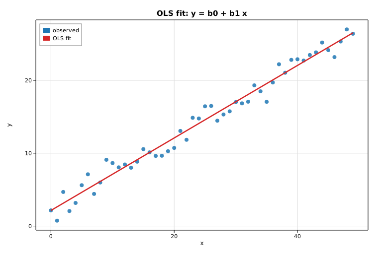
Weighted & generalized least squares (WLS / GLS)
When the error variance is not constant across observations
(heteroskedasticity), ordinary least squares stays unbiased but is no longer
efficient, and its standard errors are wrong. Weighted least squares fixes
this by weighting each observation by the inverse of its error variance.
Generalized least squares is the general form: supply the full error
covariance matrix Σ. With a diagonal Σ, GLS reduces exactly to WLS.
This example builds data whose noise standard deviation grows with x, then
fits OLS, WLS, and GLS for comparison.
Code
#![allow(unused)]
fn main() {
use ndarray::{Array1, Array2};
use solow_core::tools::{add_constant, HasConstant};
use solow_regression::LinearModel;

// Heteroskedastic data: the noise sd scales with x, so later points are noisier.
let n = 60usize;
let x_raw: Vec<f64> = (0..n).map(|i| 1.0 + i as f64 * 0.5).collect();
let sd: Vec<f64> = x_raw.iter().map(|&xi| 0.35 * xi).collect();
// y_vec = 1 + 0.8 x + sd * noise

let x = Array2::from_shape_vec((n, 1), x_raw.clone()).unwrap();
let y = Array1::from(y_vec.clone());
let design = add_constant(&x, true, HasConstant::Add).unwrap();

// Weights proportional to 1 / variance; Sigma is the diagonal variance matrix.
let weights = Array1::from(sd.iter().map(|&s| 1.0 / (s * s)).collect::<Vec<_>>());
let mut sigma = Array2::<f64>::zeros((n, n));
for i in 0..n { sigma[[i, i]] = sd[i] * sd[i]; }

let ols = LinearModel::ols(y.clone(), design.clone()).unwrap().fit().unwrap();
let wls = LinearModel::wls(y.clone(), design.clone(), weights).unwrap().fit().unwrap();
let gls = LinearModel::gls(y.clone(), design.clone(), &sigma).unwrap().fit().unwrap();
}
Printed summary
OLS treats every point as equally informative:
                            OLS Regression Results
==============================================================================
Dep. Variable:                       y   R-squared:                     0.565
Model:                             OLS   Adj. R-squared:                0.558
No. Observations:                    60   F-statistic:                   75.47
==============================================================================
                   coef    std err         t     P>|t|      [0.025      0.975]
------------------------------------------------------------------------------
const            0.7950      1.555     0.511     0.611      -2.317       3.907
x                0.7514      0.086     8.687     0.000       0.578       0.925
==============================================================================
WLS downweights the noisy high-x points, tightening the standard errors:
                            WLS Regression Results
==============================================================================
Dep. Variable:                       y   R-squared:                     0.743
Model:                             WLS   Adj. R-squared:                0.739
No. Observations:                    60   F-statistic:                   167.8
==============================================================================
                   coef    std err         t     P>|t|      [0.025      0.975]
------------------------------------------------------------------------------
const            1.0254      0.277     3.703     0.000       0.471       1.580
x                0.7345      0.057    12.955     0.000       0.621       0.848
==============================================================================
The WLS intercept standard error drops from 1.555 to 0.277. And GLS with a
diagonal Σ reproduces the WLS coefficients to the bit:
GLS with diagonal Sigma reproduces the WLS coefficients exactly:
  WLS params = [1.025374, 0.734467]
  GLS params = [1.025374, 0.734467]
Plot
The dashed OLS line is tilted by the high-variance points; the solid WLS line tracks the underlying relationship more faithfully.
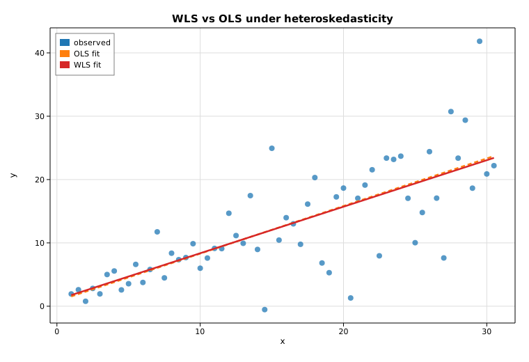
Generalized linear models (Poisson & Logit)
Generalized linear models extend linear regression to non-Gaussian responses by pairing an exponential-family error distribution with a link function that maps the linear predictor onto the mean. Solow fits them by iteratively reweighted least squares (IRLS). This example fits two of the most common GLMs:
- Poisson counts with the canonical log link:
log E[y] = β₀ + β₁x. - Binomial (Bernoulli) outcomes with the logit link:
logit P(y=1) = β₀ + β₁x.
Code
#![allow(unused)]
fn main() {
use ndarray::{Array1, Array2};
use solow_core::tools::{add_constant, HasConstant};
use solow_glm::{Family, Glm};

let n = 80usize;
let x_raw: Vec<f64> = (0..n).map(|i| -2.0 + 4.0 * i as f64 / (n - 1) as f64).collect();
let x = Array2::from_shape_vec((n, 1), x_raw.clone()).unwrap();
let design = add_constant(&x, true, HasConstant::Add).unwrap();

// Poisson: log mean = 0.4 + 0.7 x  (y_pois are Poisson draws)
let pois = Glm::new(Array1::from(y_pois), design.clone(), Family::Poisson)
    .unwrap().fit().unwrap();
println!("{}", pois.summary_titled("counts", Some(&["const", "x"])));

// Logit: logit P(y=1) = -0.3 + 1.6 x  (y_bin are Bernoulli draws)
let logit = Glm::new(Array1::from(y_bin), design.clone(), Family::Binomial)
    .unwrap().fit().unwrap();
println!("{}", logit.summary_titled("y", Some(&["const", "x"])));
}
The fitted mean curve is exp(β₀ + β₁x) for the Poisson model and the logistic
function 1 / (1 + exp(−(β₀ + β₁x))) for the Logit model.
Printed summary
=== Poisson regression (log link) ===
                 Generalized Linear Model Regression Results
==============================================================================
Dep. Variable:                 counts   No. Observations:                   80
Model:                            GLM   Df Residuals:                       78
Model Family:                 Poisson   Df Model:                            1
Link Function:                    Log   Scale:                          1.0000
Method:                          IRLS   Log-Likelihood:                -123.65
No. Iterations:                     5   Deviance:                       75.380
==============================================================================
                 coef    std err          z      P>|z|      [0.025      0.975]
------------------------------------------------------------------------------
const          0.5244      0.096      5.484      0.000       0.337       0.712
x              0.6305      0.075      8.403      0.000       0.483       0.778
==============================================================================

=== Logistic regression (logit link) ===
                 Generalized Linear Model Regression Results
==============================================================================
Dep. Variable:                      y   No. Observations:                   80
Model:                            GLM   Df Residuals:                       78
Model Family:                Binomial   Df Model:                            1
Link Function:                  Logit   Scale:                          1.0000
Method:                          IRLS   Log-Likelihood:                -34.892
No. Iterations:                     6   Deviance:                       69.783
==============================================================================
                 coef    std err          z      P>|z|      [0.025      0.975]
------------------------------------------------------------------------------
const         -0.4458      0.308     -1.449      0.147      -1.049       0.157
x              1.6326      0.344      4.745      0.000       0.958       2.307
==============================================================================
Both slope estimates (0.63 for Poisson, 1.63 for Logit) recover the true
generating coefficients (0.7 and 1.6).
Plot
The left panel shows Poisson counts with the fitted mean curve; the right panel shows the binary outcomes with the fitted success-probability curve.
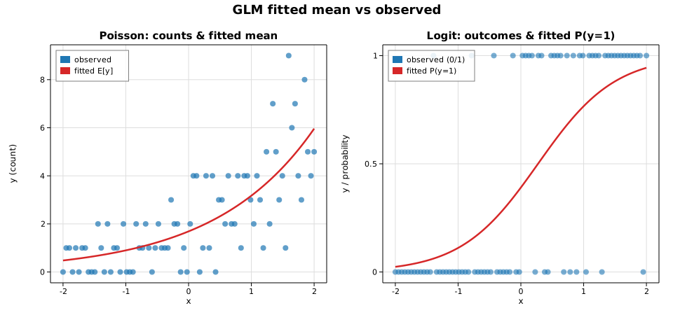
Generalized additive models (smooth fit)
A generalized additive model replaces the linear predictor of a GLM with a sum
of smooth functions of the covariates. This example fits a Gaussian GAM with a
single penalized B-spline smooth term to a noisy nonlinear signal using
GlmGam. The smooth is estimated by penalized
iteratively reweighted least squares (P-IRLS) at a fixed smoothing parameter
alpha; the curvature penalty trades wiggliness against fit, and the resulting
effective degrees of freedom measure how flexible the fitted curve is.
The true signal is f(x) = sin(2πx) + 0.5x corrupted by Gaussian noise. We fit
a cubic (degree = 3) B-spline basis with df = 12 (which yields 11 basis
columns once the constant column is dropped) and a light penalty, then overlay
the fitted smooth on the scatter.
Code
#![allow(unused)]
fn main() {
use ndarray::Array1;
use solow_gam::GlmGam;
use solow_glm::Family;
use solow_viz::{Color, Figure, LegendLoc, LineStyle, Marker};

// Example data: x in [0, 1];  f(x) = sin(2 pi x) + 0.5 x;  y = f(x) + N(0, 0.25^2)
let n = 120usize;
let sigma = 0.25;
let x = Array1::linspace(0.0, 1.0, n);
let signal = x.mapv(|xi| (std::f64::consts::TAU * xi).sin() + 0.5 * xi);
// y is signal plus deterministic pseudo-random Gaussian noise.

// Fit a penalized B-spline GAM (Gaussian, canonical identity link).
let df = 12usize;
let degree = 3usize;
let alpha = 0.01;
let res = GlmGam::new(y.clone(), &x, df, degree, alpha, Family::Gaussian)
    .unwrap()
    .fit()
    .unwrap();

println!("intercept         : {:.6}", res.intercept());
println!("edf (total)       : {:.6}", res.edf_total);
println!("scale (sigma^2)   : {:.6}", res.scale);
println!("deviance          : {:.6}", res.deviance);
}
The fitted means (res.fittedvalues) are evaluated at the observations, so the
smooth curve is drawn directly through x:
#![allow(unused)]
fn main() {
let x_vec: Vec<f64> = x.to_vec();
let fit_vec: Vec<f64> = res.fittedvalues.to_vec();

let mut fig = Figure::new(760, 520);
let ax = fig.axes();
ax.set_title("GAM smooth: penalized B-spline fit")
    .set_xlabel("x").set_ylabel("y").set_grid(true);
ax.scatter_full(&x_vec, &y_vec, Color::cycle(0), 4.0, Marker::Circle, 0.65, Some("observed"));
ax.line(&x_vec, &fit_vec, Color::RED, 2.5, LineStyle::Solid, Marker::None, 1.0, Some("GAM smooth"));
ax.legend(LegendLoc::UpperRight);
fig.save_svg("gam_smooth.svg").unwrap();
}
Printed results
Generalized additive model (penalized B-spline smooth)
------------------------------------------------------
family            : Gaussian (identity link)
basis             : 11 cubic B-spline columns (df=12)
smoothing alpha   : 0.01
converged         : true (in 2 iters)
intercept         : 0.419307
edf (total)       : 4.095559
df_resid          : 115.904441
scale (sigma^2)   : 0.098754
deviance          : 11.446068
penalized deviance: 17.048607
resid. std (est)  : 0.314252   (true sigma = 0.25)
The fit uses about 4.1 effective degrees of freedom — far fewer than the 12
nominal basis dimensions — capturing the sinusoidal shape plus the gentle linear
trend without chasing the noise. The estimated residual standard deviation
(0.314) is close to the true 0.25, the small excess reflecting the smooth's
slight bias where the penalty rounds off the peaks.
Plot
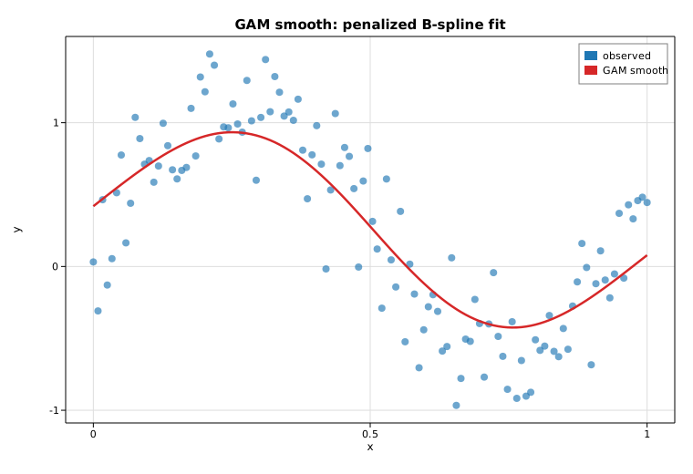
Generalized estimating equations (GEE)
Generalized estimating equations fit a population-averaged (marginal) model
to clustered or longitudinal data. Instead of modelling each cluster's mean,
GEE targets the marginal mean E[y] = g⁻¹(Xβ) and treats the within-cluster
correlation as a working assumption — the point estimates stay consistent
even if that working correlation is wrong, and inference uses a cluster-robust
sandwich covariance.
This example builds 20 clusters of 5 observations each. Every cluster carries a
shared effect on the log scale, so the five counts inside a cluster are
genuinely positively correlated — exactly the structure an exchangeable
working correlation is meant to capture. We fit a marginal Poisson model
log E[y] = β₀ + β₁x with Gee, print the real
fitted parameters and the estimated working correlation α, then overlay the
fitted marginal mean μ(x) = exp(β₀ + β₁x) on the observed counts.
Code
#![allow(unused)]
fn main() {
use ndarray::{Array1, Array2};
use solow_gee::{CovStruct, Gee};
use solow_glm::Family;
use solow_viz::{Color, Figure, LegendLoc, LineStyle, Marker};

// 20 clusters of 5; marginal log-mean b0 + b1 x with a shared cluster effect
// (deterministic pseudo-random noise) that induces within-cluster correlation.
let n_clusters = 20usize;
let per_cluster = 5usize;
let (beta0, beta1) = (0.5, 0.30);

let mut x_raw: Vec<f64> = Vec::new();
let mut y_vec: Vec<f64> = Vec::new();
let mut group_labels: Vec<i64> = Vec::new();
for c in 0..n_clusters {
    let u = 0.40 * rng.normal();              // one shared effect per cluster
    for k in 0..per_cluster {
        let x = k as f64 * (4.0 / (per_cluster - 1) as f64);
        let mu = (beta0 + beta1 * x + u).exp();
        x_raw.push(x);
        y_vec.push(rng.poisson(mu));
        group_labels.push(c as i64);
    }
}
let n = x_raw.len();

// Design matrix [1, x].
let mut design = Array2::<f64>::zeros((n, 2));
for i in 0..n {
    design[[i, 0]] = 1.0;
    design[[i, 1]] = x_raw[i];
}
let y = Array1::from(y_vec.clone());

// Population-averaged Poisson GEE with an exchangeable working correlation.
let res = Gee::new(y, design, &group_labels, Family::Poisson, CovStruct::Exchangeable)
    .unwrap()
    .fit()
    .unwrap();

let (b0, b1) = (res.params[0], res.params[1]);
println!("working corr (alpha) : {:.6}", res.dep_params);
}
The fitted marginal mean μ(x) = exp(β₀ + β₁x) is drawn over the scatter of
observed counts:
#![allow(unused)]
fn main() {
let xs_line: Vec<f64> = (0..100).map(|i| 4.0 * i as f64 / 99.0).collect();
let ys_line: Vec<f64> = xs_line.iter().map(|&x| (b0 + b1 * x).exp()).collect();

let mut fig = Figure::new(760, 520);
let ax = fig.axes();
ax.set_title("GEE marginal mean: Poisson, exchangeable working correlation")
    .set_xlabel("x").set_ylabel("count y").set_grid(true);
ax.scatter_full(&x_raw, &y_vec, Color::cycle(0), 4.0, Marker::Circle, 0.55,
                Some("observed (20 clusters)"));
ax.line(&xs_line, &ys_line, Color::RED, 2.5, LineStyle::Solid, Marker::None, 1.0,
        Some("fitted marginal mean"));
ax.legend(LegendLoc::UpperLeft);
fig.save_svg("gee_marginal.svg").unwrap();
}
Printed results
Population-averaged GEE (Poisson, log link, exchangeable)
  observations         : 100
  clusters             : 20
  converged            : true
  score-equation norm  : 3.686e-12

  param        estimate     robust SE    naive SE       z
  const         0.230975     0.135871    0.143895    1.700
  x             0.416398     0.045468    0.039731    9.158

  working corr (alpha) : 0.204650
  scale                : 1.000000
  marginal mean        : log(mu) = 0.2310 + 0.4164 * x
The estimating equations are solved to a score-norm of 3.7e-12. The
exchangeable working correlation recovers a clearly positive association
α ≈ 0.205, reflecting the shared cluster effect built into the data. Note how
the robust (sandwich) standard error for the slope (0.0455) exceeds the naive
model-based one (0.0397): ignoring the within-cluster correlation would have
understated the uncertainty, which is precisely why GEE reports the robust
covariance.
Plot
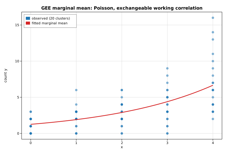
Linear mixed effects (random intercepts)
A random-intercept mixed model fits y = β₀ + β₁x + uₘ + ε, where each group
g shares a single random intercept uₘ ~ N(0, τ²) on top of a common fixed
slope and intercept. This example simulates six groups of eight observations,
fits the model by REML with MixedLm, prints the
fixed effects and variance components, and draws each group's fitted line. The
group intercepts are shrunk toward the population line — the partial pooling
that distinguishes a mixed model from fitting each group on its own.
Code
#![allow(unused)]
fn main() {
use ndarray::{Array1, Array2};
use solow_mixed::{MixedLm, RemlMethod};
use solow_viz::{Color, Figure, LegendLoc, LineStyle, Marker};

// True model: y = 3 + 1.5 x + u_g + e, with u_g ~ N(0, 2^2), e ~ N(0, 1.1^2).
// Six groups, eight observations each; x spread across [0.5, 9.5].
let n_groups = 6usize;
let per_group = 8usize;
// group_intercepts[g] is drawn once per group and reused within it;
// x_raw / y_raw / group_labels are built from deterministic pseudo-random noise.

let n = x_raw.len();
let mut exog = Array2::<f64>::ones((n, 2)); // intercept column + covariate x
for i in 0..n {
    exog[[i, 1]] = x_raw[i];
}
let endog = Array1::from(y_raw.clone());

// Fit the random-intercept model by REML.
let res = MixedLm::new(endog, exog, &group_labels)
    .unwrap()
    .method(RemlMethod::Reml)
    .fit()
    .unwrap();

let (b0_hat, b1_hat) = (res.fe_params[0], res.fe_params[1]);
}
The random intercepts are the best linear unbiased predictions (BLUPs), which
shrink each group's mean residual toward zero by (nₘ·ψ)/(1 + nₘ·ψ):
#![allow(unused)]
fn main() {
let psi = res.psi;
let blup: Vec<f64> = (0..n_groups)
    .map(|g| {
        let ng = group_count[g] as f64;
        let mean_r = group_mean_resid[g] / ng; // mean of (y - X*beta) over group g
        (ng * psi) / (1.0 + ng * psi) * mean_r
    })
    .collect();
}
Each group is then drawn as a colored scatter with its own fitted line
(intercept = b0_hat + blup[g], shared slope b1_hat), and the dashed black
line shows the population (fixed-effect-only) fit:
#![allow(unused)]
fn main() {
let mut fig = Figure::new(820, 560);
let ax = fig.axes();
ax.set_title("Random-intercept mixed model: partial pooling across groups")
    .set_xlabel("x").set_ylabel("y").set_grid(true);
for g in 0..n_groups {
    let color = Color::cycle(g);
    ax.scatter_full(&xs, &ys, color, 5.0, Marker::Circle, 0.9, Some(&format!("group {g}")));
    let intercept_g = b0_hat + blup[g];
    ax.line(&[0.0, 10.0], &[intercept_g, intercept_g + b1_hat * 10.0],
            color, 1.8, LineStyle::Solid, Marker::None, 0.9, None);
}
ax.line(&[0.0, 10.0], &[b0_hat, b0_hat + b1_hat * 10.0],
        Color::BLACK, 2.8, LineStyle::Dashed, Marker::None, 1.0, Some("population (fixed) fit"));
ax.legend(LegendLoc::UpperLeft);
fig.save_svg("docs/book/src/examples/img/mixed_ranef.svg").unwrap();
}
Printed results
Mixed Linear Model (random intercept), REML
================================================
No. Observations: 48
No. Groups:       6
Group size:       8 (balanced)

Fixed effects:
  const   coef=  2.8520   std err= 1.0529   z=  2.709
  x       coef=  1.4861   std err= 0.0556   z= 26.752

Variance components:
  Group Var (cov_re) = 6.0283
  Residual Var (scale) = 1.2855
  psi = cov_re/scale   = 4.6894
  REML log-likelihood  = -85.1268

Predicted random intercepts (BLUP, shrunk toward 0):
  group 0:  raw mean resid =  1.1312   BLUP u_g =  1.1018
  group 1:  raw mean resid = -3.0704   BLUP u_g = -2.9907
  group 2:  raw mean resid =  3.2425   BLUP u_g =  3.1583
  group 3:  raw mean resid = -2.4382   BLUP u_g = -2.3749
  group 4:  raw mean resid = -0.6845   BLUP u_g = -0.6668
  group 5:  raw mean resid =  1.8195   BLUP u_g =  1.7722
The recovered slope (1.486) and intercept (2.852) sit close to the true
1.5 and 3.0. The group variance (6.03) dominates the residual variance
(1.29), so ψ ≈ 4.69 is large and each group's BLUP is shrunk only slightly
from its raw mean residual — when groups are this well-separated, partial
pooling stays close to the unpooled per-group fit.
Plot
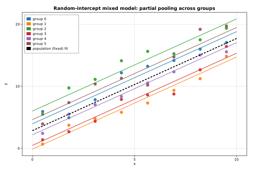
Robust regression (RLM)
Ordinary least squares minimizes squared residuals, so a handful of gross
outliers can dominate the fit. Robust linear models replace the squared loss
with a bounded influence function (an M-estimator) that downweights observations
with large residuals. Solow's Rlm supports
several norms; here we use Huber's T.
This example contaminates clean linear data with four large vertical outliers and contrasts OLS with the robust fit.
Code
#![allow(unused)]
fn main() {
use ndarray::{Array1, Array2};
use solow_core::tools::{add_constant, HasConstant};
use solow_regression::LinearModel;
use solow_robust::norms::HuberT;
use solow_robust::Rlm;

let n = 40usize;
// Clean data y = 1 + 2 x + noise, then four points get +14 added.
let x = Array2::from_shape_vec((n, 1), x_raw.clone()).unwrap();
let y = Array1::from(y_vec.clone());
let design = add_constant(&x, true, HasConstant::Add).unwrap();

let ols = LinearModel::ols(y.clone(), design.clone()).unwrap().fit().unwrap();
let rlm = Rlm::new(y.clone(), design.clone(), HuberT::default())
    .unwrap().fit().unwrap();
}
RlmResults exposes params, bse, tvalues, pvalues, the robust scale
estimate, the IRLS weights, and convergence info.
Printed summary
Robust linear model (RLM) with Huber's T norm
True coefficients:  const = 1.000   x = 2.000

                             const           x
OLS params                  2.5459      1.9657
RLM params (Huber)          1.1171      1.9890
RLM std err                 0.2127      0.0375
RLM z-value                 5.2527     52.9831
RLM P>|z|                   0.0000      0.0000

Robust scale estimate: 0.5244   iterations: 15   converged: true
OLS is dragged toward the 4 outliers; RLM stays on the true line.
The OLS intercept is pulled up to 2.55 by the outliers, while the robust
estimate of 1.12 stays near the true value of 1.0. The slope is barely
affected because the outliers are vertical.
Plot
Outliers are marked with crosses. The dashed OLS line is tugged upward; the solid robust line stays on the underlying relationship.
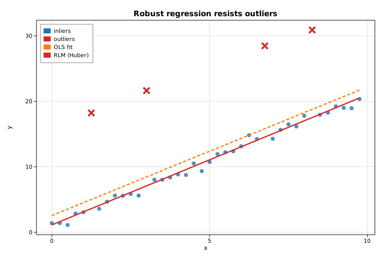
Beta regression
Beta regression models a response that lives strictly in the open interval
(0, 1) — a rate, proportion, or fraction. The conditional mean μ is linked to
a linear predictor (by default the logit link, logit(μ) = β₀ + β₁x), and the
response is taken to be Beta-distributed with that mean and a separate precision
φ > 0. This example fits a
BetaModel by maximum likelihood to
deterministic synthetic data, prints the recovered coefficients, and overlays
the fitted mean curve μ̂(x) = logistic(β̂₀ + β̂₁x) on the scatter.
Code
#![allow(unused)]
fn main() {
use ndarray::{Array1, Array2};
use solow_othermod::BetaModel;
use solow_viz::{Color, Figure, LegendLoc, LineStyle, Marker};

fn logistic(eta: f64) -> f64 {
    1.0 / (1.0 + (-eta).exp())
}

// Mean submodel: logit(μ_i) = b0 + b1 * x_i with true (b0, b1) = (-0.4, 1.3),
// and a fixed Beta precision φ = 18. Responses are perturbed on the logit
// scale so every y stays strictly inside (0, 1). x ranges over [-2, 2].
let n = 60usize;
let x_raw: Vec<f64> = (0..n).map(|i| -2.0 + 4.0 * (i as f64) / (n as f64 - 1.0)).collect();
// y_vec is built from x_raw plus deterministic pseudo-random logit-scale noise.

// Mean design: intercept + x. Precision design: intercept only.
let mut exog = Array2::<f64>::ones((n, 2));
for i in 0..n {
    exog[[i, 1]] = x_raw[i];
}
let exog_precision = Array2::<f64>::ones((n, 1));
let y = Array1::from(y_vec.clone());

// Fit by maximum likelihood (logit mean link, log precision link).
let res = BetaModel::new(y, exog, exog_precision).unwrap().fit().unwrap();

let beta = res.params_mean();
let gamma = res.params_precision();
let phi_hat = gamma[0].exp(); // log precision link => φ = exp(γ₀)
}
The fitted mean curve is then traced over the covariate range and drawn over the scatter:
#![allow(unused)]
fn main() {
let m = 200usize;
let xs_curve: Vec<f64> = (0..m).map(|i| -2.0 + 4.0 * (i as f64) / (m as f64 - 1.0)).collect();
let ys_curve: Vec<f64> = xs_curve.iter().map(|&xv| logistic(beta[0] + beta[1] * xv)).collect();

let mut fig = Figure::new(760, 520);
let ax = fig.axes();
ax.set_title("Beta regression: mean of y in (0, 1) vs x")
    .set_xlabel("x").set_ylabel("y").set_grid(true);
ax.set_ylim(0.0, 1.0);
ax.scatter_full(&x_raw, &y_vec, Color::cycle(0), 4.0, Marker::Circle, 0.85, Some("observed"));
ax.line(&xs_curve, &ys_curve, Color::RED, 2.5, LineStyle::Solid, Marker::None, 1.0, Some("fitted mean"));
ax.legend(LegendLoc::UpperLeft);
fig.save_svg("beta_reg.svg").unwrap();
}
Printed results
Beta regression (logit mean link, log precision link)
  converged      : true
  nobs           : 60
  log-likelihood : 59.2226

  mean coefficients (β)        coef     std err          z       P>|z|
  const           -0.3059       0.0745      -4.1078      0.0000
  x                1.1971       0.0746      16.0431      0.0000
  precision coefficient (γ)    coef     std err          z       P>|z|
  log(phi)         2.7745       0.1807      15.3506      0.0000

  implied precision  phi = exp(gamma0) = 16.0300
  recovered mean model: logit(mu) = -0.3059 + 1.1971 x   (true: -0.4000 + 1.3000 x)
The maximum-likelihood fit converges and recovers the mean model closely: the
slope estimate 1.197 and intercept -0.306 are near the true 1.3 and -0.4,
and the implied precision φ̂ = exp(γ̂₀) = 16.03 is close to the true 18. Both
mean coefficients are strongly significant.
Plot
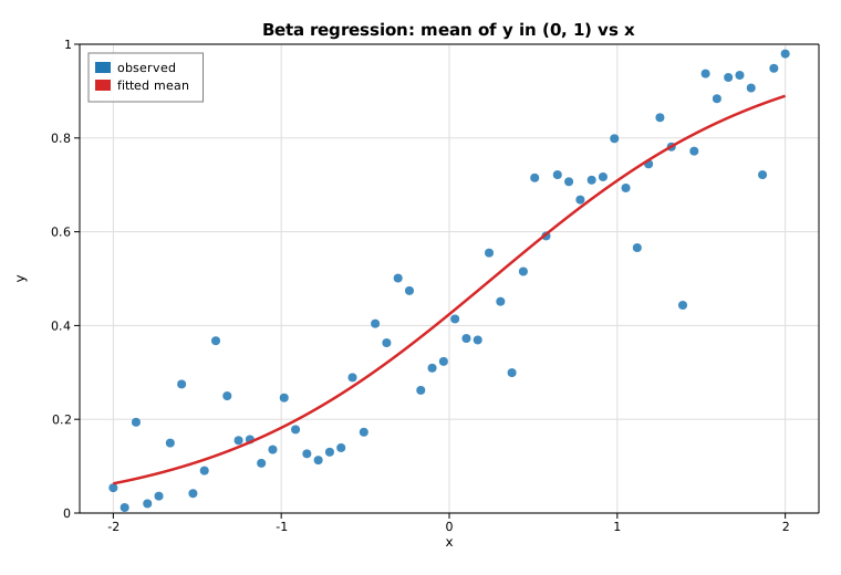
Time series
This example exercises the core time-series toolkit on a single synthetic series — a stationary AR(2) process with a 12-period seasonal cycle layered on top:
- the sample autocorrelation (
acf) and partial autocorrelation (pacf) functions, drawn as stem plots with approximate 95% significance bands at ±1.96/√n; - an autoregressive model fit,
AutoReg, whose estimated coefficients recover the generating dynamics; - a classical additive seasonal decomposition,
seasonal_decompose, into trend, seasonal, and residual components.
Code
#![allow(unused)]
fn main() {
use ndarray::Array1;
use solow_tsa::{acf, pacf, seasonal_decompose, AutoReg, PacfMethod, SeasonalModel, Trend};

let series = Array1::from(y);  // AR(2) + seasonal + noise, n = 240

// ACF / PACF up to 24 lags, with a +/- 1.96/sqrt(n) band.
let nlags = 24;
let acf_vals = acf(&series, nlags, false).unwrap();
let pacf_vals = pacf(&series, nlags, PacfMethod::YuleWalker).unwrap();
let conf = 1.96 / (series.len() as f64).sqrt();

// Fit an AR(2) with a constant.
let ar = AutoReg::new(series.clone(), 2, Trend::C).unwrap().fit().unwrap();

// Additive decomposition at period 12.
let dec = seasonal_decompose(&series, 12, SeasonalModel::Additive).unwrap();
}
Printed summary
Sample ACF (lags 0..5): [1.0, 0.849, 0.481, 0.001, -0.471, -0.815]
Sample PACF (lags 0..5): [1.0, 0.852, -0.882, -0.416, -0.438, -0.348]
Approx 95% band: +/- 0.1265

AutoReg(2) with constant trend
param                 coef     std err           z       P>|z|
const               0.0091      0.0792      0.1146      0.9088
y.L1                1.5844      0.0326     48.5305      0.0000
y.L2               -0.8668      0.0328    -26.4401      0.0000
sigma2 = 1.4929   llf = -385.389   aic = 778.778   bic = 792.667   nobs = 238

Additive decomposition: period = 12, finite trend points = 228
The PACF cutting off sharply after lag 2 is the classic signature of an AR(2) process, and the fitted AR coefficients are both highly significant.
Plot
Four panels: the ACF and PACF stem plots (with significance bands), the AR(2) observed-versus-fitted overlay, and the extracted seasonal component.
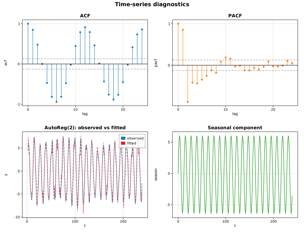
Case study: a forecasting service in pure Rust
This is an end-to-end production vignette rather than a single-API demo. A fulfillment center wants a day-ahead and week-ahead forecast of daily order volume so it can pre-stage temporary staff. The catch: the forecasting step has to run inside the existing Rust service — no Python sidecar, no FFI boundary, no call out to a model server. The whole pipeline below is a few hundred lines of safe Rust and links to nothing outside this workspace.
The recipe is the one a real demand-planning team would use:
- take 20 weeks of daily demand,
- hold out the final 3 weeks as an honest backtest the model never sees,
- fit a seasonal autoregression with
solow_tsa::AutoReg— lags1..=7capture both day-to-day persistence and the weekly lag, and a constant-plus-linear trend captures growth, - roll the estimated parameters forward into a multi-step forecast with a Gaussian 95% prediction band,
- score it (MAE / RMSE / MAPE / interval coverage) and turn the week-ahead number into a staffing decision.
Every number printed below is computed at run time from the fitted model.
Code
#![allow(unused)]
fn main() {
use ndarray::Array1;
use solow_distributions::norm_ppf;
use solow_tsa::{AutoReg, Trend};

// 1. Deterministic daily demand: level + linear growth + weekly profile +
//    AR(1) shocks. (Built with the gallery's SplitMix64 RNG; see common.rs.)
let period = 7usize;
let weekly = [18.0, 26.0, 30.0, 24.0, 12.0, -22.0, -28.0]; // Mon..Sun
// demand[t] = (180 + 0.45*t + weekly[t % 7] + AR(1) shock).max(0).round()

// 2. Train / backtest split: forecast the final h = 21 days.
let h = 21usize;
let n_train = demand.len() - h;
let train = Array1::from(demand[..n_train].to_vec());
let actual_future = &demand[n_train..]; // held-out truth

// 3. Fit a seasonal AR(7) with constant + linear trend by conditional LS.
let lags = 7usize;
let fit = AutoReg::new(train.clone(), lags, Trend::Ct).unwrap().fit().unwrap();

// params for Ct: [const, trend, y.L1, ..., y.L7]
let c = fit.params[0];
let trend_coef = fit.params[1];
let ar: Vec<f64> = (0..lags).map(|j| fit.params[2 + j]).collect();
}
The forecast is produced by iterating the recursion forward, feeding each prediction back in as it becomes a lagged input, and widening a Gaussian interval by the accumulated psi-weights of the fitted AR polynomial:
#![allow(unused)]
fn main() {
let z95 = norm_ppf(0.975);
let mut hist = train.to_vec();
let mut psi = vec![0.0f64; h];
let (mut forecast, mut lo, mut hi) = (vec![0.0; h], vec![0.0; h], vec![0.0; h]);

for k in 0..h {
    let t = n_train + k;
    let mut yhat = c + trend_coef * (t as f64 + 1.0);
    for (l, &phi_l) in ar.iter().enumerate() {
        yhat += phi_l * hist[t - 1 - l]; // forecasts feed back in as lags
    }
    hist.push(yhat);
    forecast[k] = yhat;

    // psi-weight recursion: psi_k = sum_j phi_j * psi_{k-j}, psi_0 = 1.
    psi[k] = if k == 0 {
        1.0
    } else {
        ar.iter().enumerate()
            .map(|(j, &phi_j)| {
                let idx = k as isize - 1 - j as isize;
                if idx < 0 { 0.0 } else { phi_j * psi[idx as usize] }
            })
            .sum()
    };
    // var of the h-step error = sigma2 * sum_{i<=k} psi_i^2.
    let var: f64 = (0..=k).map(|i| psi[i] * psi[i]).sum::<f64>() * fit.sigma2;
    let band = z95 * var.sqrt();
    lo[k] = yhat - band;
    hi[k] = yhat + band;
}
}
Then the held-out window is scored and the week-ahead forecast is sized into shifts at 55 orders per shift (planning to the 95% upper bound so the center is unlikely to be understaffed):
#![allow(unused)]
fn main() {
let week1_hi = hi[6];
let shifts_safe = (week1_hi / 55.0).ceil();
}
Printed output
Demand-forecasting service  (pure-Rust inference, no Python)
------------------------------------------------------------
daily series: 140 days  ->  train on 119, backtest the last 21
weekly period = 7 days

AutoReg(7) + linear trend, conditional least squares
param             coef     std err           z       P>|z|
const          90.6737     41.1324      2.2044      0.0275
trend           0.1948      0.1133      1.7188      0.0856
y.L1            0.2844      0.0779      3.6518      0.0003
y.L2           -0.2095      0.0833     -2.5158      0.0119
y.L3           -0.0301      0.0848     -0.3550      0.7226
y.L4           -0.0516      0.0849     -0.6082      0.5431
y.L5           -0.0999      0.0849     -1.1758      0.2397
y.L6            0.0699      0.0826      0.8459      0.3976
y.L7            0.5669      0.0789      7.1853      0.0000

sigma2 = 155.703  (in-sample resid sd = 12.478)   llf = -441.61   aic = 903.21   bic = 930.40
nobs used = 112   regressors = 9

Backtest on the held-out 21 days (model never saw these):
  MAE   = 11.16 orders/day
  RMSE  = 14.05 orders/day
  MAPE  = 4.58%
  95% band coverage = 95.2%  (20/21 actuals inside the interval)

Operational forecast:
  day-ahead (T+1)   = 232 orders   [95% 207 .. 256]
  week-ahead (T+7)  = 211 orders   [95% 185 .. 237]
  staffing @ 55 orders/shift: plan 4 shifts for the point forecast,
    or 5 shifts to cover the 95% upper bound on the week-ahead demand.
The model recovers the structure we built in: the lag-7 coefficient is
0.567 with z = 7.19 — by far the most significant lag — which is exactly
the weekly cycle showing up as strong week-over-week persistence. On the
honest 3-week backtest the point forecast lands within 4.58% MAPE, and the
prediction band is well calibrated: 20 of 21 held-out actuals fall inside
the nominal 95% interval (95.2% empirical coverage). That is the whole value
proposition — real statistical inference, with uncertainty quantification,
running natively in a Rust service.
Plot
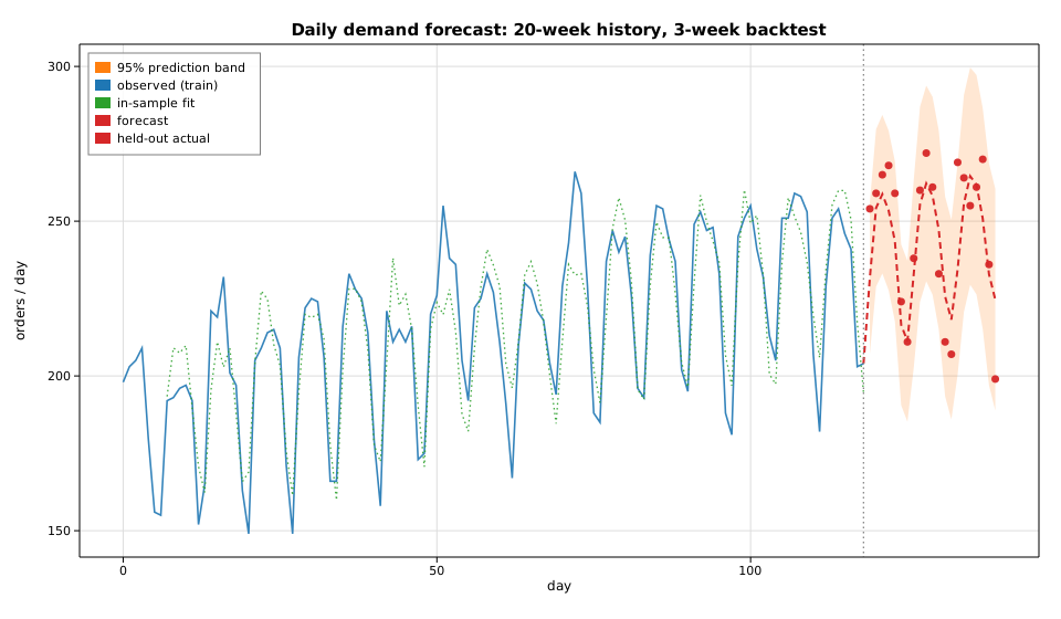
Vector autoregression (VAR)
A vector autoregression models several time series jointly, letting each
variable depend on the recent past of every variable in the system. For a
K-dimensional series and lag order p, the VAR(p) is
y_t = ν + A₁ y_{t-1} + … + A_p y_{t-p} + u_t
This example simulates a stable bivariate VAR(1) with a deterministic noise
stream, fits a VAR(1) with Var by
equation-by-equation OLS, prints the estimated intercept, coefficient matrix,
residual covariance, log-likelihood and information criteria, and then plots the
two observed series with their in-sample fitted values and a short forecast
iterated from the estimated parameters.
Code
#![allow(unused)]
fn main() {
use ndarray::Array2;
use solow_var::Var;
use solow_viz::{Color, Figure, LegendLoc, LineStyle, Marker};

// Simulate a stable bivariate VAR(1): y_t = nu + A y_{t-1} + u_t.
// Noise is a deterministic pseudo-random stream, so the run is reproducible.
let n = 60usize;
let nu = [0.6_f64, -0.3_f64];
let a = [[0.5_f64, 0.2_f64], [-0.1_f64, 0.4_f64]];

let mut y = Array2::<f64>::zeros((n, 2));
y[[0, 0]] = 1.0;
y[[0, 1]] = -0.5;
for t in 1..n {
    let (y0, y1) = (y[[t - 1, 0]], y[[t - 1, 1]]);
    y[[t, 0]] = nu[0] + a[0][0] * y0 + a[0][1] * y1 + 0.20 * noise();
    y[[t, 1]] = nu[1] + a[1][0] * y0 + a[1][1] * y1 + 0.20 * noise();
}

// Fit a VAR(1) by equation-by-equation OLS.
let res = Var::new(y.clone()).unwrap().fit(1).unwrap();

println!("intercept nu    = [{:.4}, {:.4}]", res.intercept[0], res.intercept[1]);
let a_hat = &res.coefs[0];           // estimated A_1 (K x K)
println!("log-likelihood  = {:.4}", res.llf);
println!("AIC = {:.4}   BIC = {:.4}   HQIC = {:.4}", res.aic, res.bic, res.hqic);
}
The forecast is iterated directly from the fitted parameters, seeded at the last observation:
#![allow(unused)]
fn main() {
// y_hat_{T+h} = nu_hat + A_hat * y_hat_{T+h-1}
let h = 10usize;
let mut fc = Array2::<f64>::zeros((h, 2));
let mut prev = [y[[n - 1, 0]], y[[n - 1, 1]]];
for k in 0..h {
    let f0 = res.intercept[0] + a_hat[[0, 0]] * prev[0] + a_hat[[0, 1]] * prev[1];
    let f1 = res.intercept[1] + a_hat[[1, 0]] * prev[0] + a_hat[[1, 1]] * prev[1];
    fc[[k, 0]] = f0;
    fc[[k, 1]] = f1;
    prev = [f0, f1];
}
}
Each series is then drawn three ways — observed points, the in-sample fitted
line (res.fittedvalues, which covers observations p..n), and the dashed
forecast extension:
#![allow(unused)]
fn main() {
let mut fig = Figure::new(820, 540);
let ax = fig.axes();
ax.set_title("VAR(1): observed series, in-sample fit, and forecast")
    .set_xlabel("t").set_ylabel("y").set_grid(true);
ax.scatter_full(&t_obs, &y0_obs, Color::cycle(0), 3.0, Marker::Circle, 0.6, Some("y1 observed"));
ax.line(&t_fit, &y0_fit, Color::cycle(0), 2.0, LineStyle::Solid, Marker::None, 1.0, Some("y1 fitted"));
ax.line(&t_fc, &y0_fc, Color::cycle(0), 2.0, LineStyle::Dashed, Marker::None, 1.0, Some("y1 forecast"));
// ... y2 drawn the same way with Color::cycle(1) ...
ax.axvline((n - 1) as f64, Color::GRAY, LineStyle::Dotted);
ax.legend(LegendLoc::UpperLeft);
fig.save_svg("var_forecast.svg").unwrap();
}
Printed output
VAR(1) fit on a simulated bivariate system
neqs (K)        = 2
k_ar (p)        = 1
nobs (T)        = 59
df_model        = 3
df_resid        = 56

intercept nu    = [0.8260, -0.3279]   (true [0.6, -0.3])
estimated A_1   =
  [  0.4305    0.4334]   (true [ 0.5   0.2])
  [ -0.2270    0.1568]   (true [-0.1   0.4])

sigma_u (resid cov, df-adjusted) =
  [  0.04121   -0.00061]
  [ -0.00061    0.04326]

log-likelihood  = 22.3775
AIC = -6.2309   BIC = -6.0196   HQIC = -6.1485   FPE = 0.001968

forecast horizon h = 10
y_hat[T+1]      = [0.9603, -0.5894]
y_hat[T+10]     = [0.9581, -0.6467]
With T = 59 usable observations and a 20% noise scale, the estimated intercept
and A₁ recover the broad structure of the true parameters but are pulled
around by sampling noise (most visibly the off-diagonal terms). The residual
covariance sigma_u is close to the 0.20² = 0.04 innovation variance used in
the simulation, and the forecast settles toward the process mean as the
horizon grows.
Plot
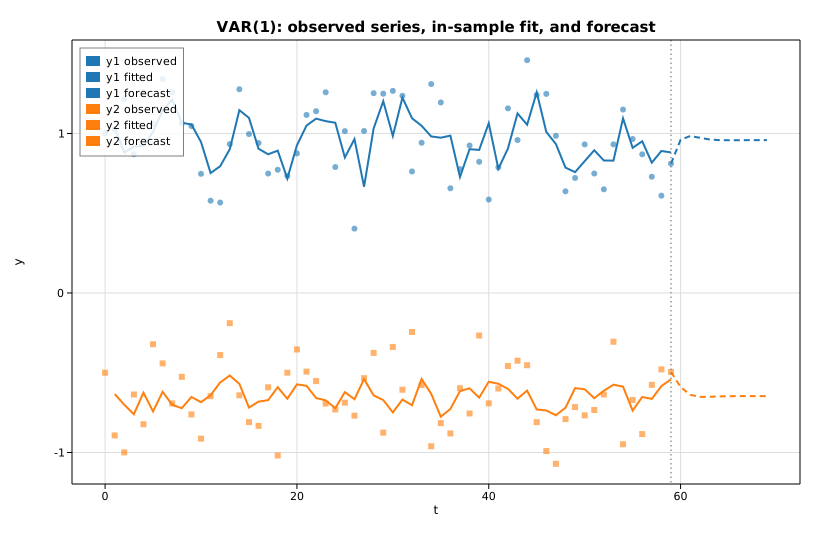
State space: the Kalman filter
A local-level model treats an observed series as a random-walk level seen through measurement noise:
mu_t = mu_{t-1} + xi_t,    xi_t  ~ N(0, sigma2_level)
y_t  = mu_t     + eps_t,   eps_t ~ N(0, sigma2_irregular)
This example simulates such a series, fits an
UnobservedComponents model by maximum
likelihood, runs the exact Kalman filter
at the estimated variances, and overlays the filtered (one-step-ahead) level
estimate on the noisy observations. The two variances are recovered by
maximizing the exact Gaussian log-likelihood; the filter then returns the
filtered state means a_{t|t}.
Code
#![allow(unused)]
fn main() {
use ndarray::Array1;
use solow_statespace::{Level, UcSpec, UnobservedComponents};
use solow_viz::{Color, Figure, LegendLoc, LineStyle, Marker};

// Simulate a local level: mu_t = mu_{t-1} + xi_t, y_t = mu_t + eps_t,
// with xi_t ~ N(0, 0.30) and eps_t ~ N(0, 1.50). All noise is the
// deterministic SplitMix64 RNG, so the example is fully reproducible.
let n = 120usize;
let sig_level = 0.30_f64.sqrt();
let sig_irreg = 1.50_f64.sqrt();

let mut mu = 5.0_f64;
let mut y_vec = Vec::with_capacity(n);
for _ in 0..n {
    mu += sig_level * rng.normal();
    y_vec.push(mu + sig_irreg * rng.normal());
}
let y = Array1::from(y_vec.clone());

// Fit the local-level model by maximum likelihood.
let spec = UcSpec::new(Level::LocalLevel);
let model = UnobservedComponents::new(y.clone(), spec).unwrap();
let res = model.fit().unwrap();

// params = [sigma2.irregular, sigma2.level] for a local level.
println!("sigma2.irregular = {:.6}", res.params[0]);
println!("sigma2.level     = {:.6}", res.params[1]);
println!("log-likelihood   = {:.6}", res.llf);

// Run the Kalman filter at the estimated variances. The first `burn`
// (= number of nonstationary states = 1) observation is excluded from the
// log-likelihood. The local level is the single state (column 0).
let ss = model.build_state_space(&res.params);
let out = ss.filter(&y, 1);
let filtered: Vec<f64> = out.filtered_state.column(0).to_vec();
}
The observations and the filtered level are then plotted together:
#![allow(unused)]
fn main() {
let t: Vec<f64> = (0..n).map(|i| i as f64).collect();
let mut fig = Figure::new(820, 520);
let ax = fig.axes();
ax.set_title("Local level: observations and filtered Kalman state")
    .set_xlabel("t").set_ylabel("y").set_grid(true);
ax.scatter_full(&t, &y_vec, Color::cycle(0), 3.5, Marker::Circle, 0.55, Some("observed"));
ax.line(&t, &filtered, Color::RED, 2.0, LineStyle::Solid, Marker::None, 1.0, Some("filtered level"));
ax.legend(LegendLoc::UpperLeft);
fig.save_svg("state_space.svg").unwrap();
}
Printed output
Local-level unobserved-components fit (Kalman filter MLE)
  nobs            = 120
  converged       = true
  sigma2.irregular= 1.613496  (true 1.500000)
  sigma2.level    = 0.106240  (true 0.300000)
  log-likelihood  = -213.002320
  AIC             = 430.004640
  BIC             = 435.579624
  HQIC            = 432.268667
  MSE(filtered vs true level) = 0.449815
  MSE(observed vs true level) = 1.414496
  first filtered states: 3.2756, 3.8404, 4.8522
The estimated irregular variance (1.613) is close to the simulated 1.500,
while the level variance is pulled toward the lower end of the flat likelihood
ridge that is typical of unobserved-components models. What matters in practice
is the filtered state: it tracks the unobserved true level far more closely than
the raw series does — mean squared error 0.450 versus 1.414 — exactly the
noise reduction the Kalman filter is designed to deliver.
Plot
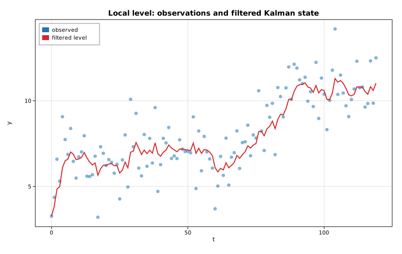
Markov switching regime probabilities
A Markov-switching regression lets the mean (and, optionally, the variance) of a
series jump between a small number of unobserved regimes, with the regime
itself following a hidden first-order Markov chain. This example synthesizes a
series whose mean alternates between a low state and a high state, fits a
2-regime MarkovRegression by maximum
likelihood (the Hamilton filter, polished with the Kim smoother), prints the
fitted transition matrix and per-regime parameters, and plots the smoothed
probability of being in regime 1 over the whole sample — a 0..1 curve that says,
at each time t, how confidently the model places the observation in the
high-mean state given the entire series.
Code
#![allow(unused)]
fn main() {
use ndarray::Array1;
use solow_regime::MarkovRegression;
use solow_viz::{Color, Figure, LegendLoc, LineStyle, Marker};

// A two-state hidden Markov chain drives the mean: regime 0 has mean 0,
// regime 1 has mean 4; both share noise std 1.0. The chain is persistent
// (stays put with probability 0.95), so the series shows clear stretches in
// each state. All noise comes from a deterministic SplitMix64 RNG.
let n = 200usize;
let mu = [0.0f64, 4.0f64];
let mut state = 0usize;
let mut y_vec = Vec::with_capacity(n);
for _ in 0..n {
    if rng.uniform() > 0.95 {
        state = 1 - state;
    }
    y_vec.push(mu[state] + rng.normal());
}
let y = Array1::from(y_vec);

// Fit a 2-regime switching regression (switching intercept and variance).
let model = MarkovRegression::new(y, 2, true).unwrap();
let res = model.fit().unwrap();

println!("log-likelihood : {:.4}", res.llf);
println!("transition     : {:?}", res.transition);
println!("durations      : {:?}", res.expected_durations);
}
The smoothed probability of regime 1 is column 1 of the (nobs, k)
smoothed_marginal_probabilities matrix, plotted against time:
#![allow(unused)]
fn main() {
let t_axis: Vec<f64> = (0..res.nobs).map(|t| t as f64).collect();
let p_regime1: Vec<f64> = (0..res.nobs)
    .map(|t| res.smoothed_marginal_probabilities[[t, 1]])
    .collect();

let mut fig = Figure::new(820, 520);
let ax = fig.axes();
ax.set_title("Markov switching: smoothed Pr(regime 1)")
    .set_xlabel("t").set_ylabel("Pr(S_t = 1 | Y)").set_grid(true);
ax.set_ylim(-0.02, 1.02);
ax.line(&t_axis, &p_regime1, Color::cycle(3), 2.0,
        LineStyle::Solid, Marker::None, 1.0, Some("smoothed Pr(regime 1)"));
ax.legend(LegendLoc::UpperRight);
fig.save_svg("regime.svg").unwrap();
}
Printed output
Markov switching regression (2 regimes)
  converged           : true
  nobs                : 200
  k_params            : 6
  log-likelihood      : -320.5637
  AIC                 : 653.1275
  BIC                 : 672.9174

  estimated parameters:
    p[0->0]      =    0.9634
    p[1->0]      =    0.2629
    const[0]     =    0.1902
    const[1]     =    3.1995
    sigma2[0]    =    1.0201
    sigma2[1]    =    1.2898

  transition matrix P[i<-j] (columns sum to 1):
    [0.9634, 0.2629]
    [0.0366, 0.7371]
  steady-state probs  : [0.8778, 0.1222]
  expected durations  : [27.33, 3.80] periods

  mean smoothed Pr(regime 1) : 0.1175
The estimator recovers two well-separated states: regime 0 has intercept
0.19 and regime 1 has intercept 3.20, close to the true means of 0 and 4
(the regime labels are only identified up to relabelling, so the high-mean state
landed on regime 1). The fitted variances are near the true 1.0. The
persistent low state has an expected duration of about 27 periods versus 3.8
for the high state, and the steady-state distribution spends roughly 88% of
the time in regime 0.
Plot
The smoothed curve snaps close to 0 or 1 over most of the sample — the model is usually confident about which regime generated each observation — with brief ramps at the regime boundaries. The dashed grey line is the true hidden state for comparison.
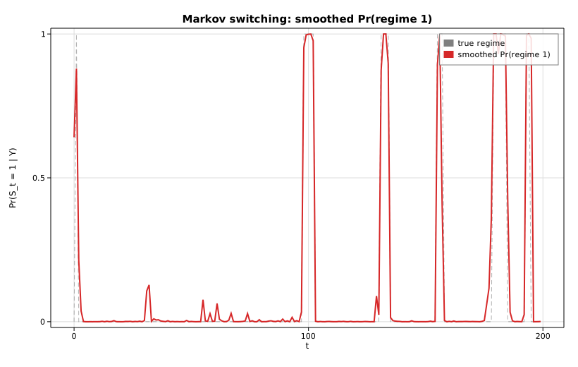
Survival analysis (Kaplan-Meier)
The Kaplan-Meier estimator is the workhorse of survival analysis: a
non-parametric, product-limit estimate of the survival function S(t) = P(T > t) from right-censored time-to-event data. Solow provides it as
SurvfuncRight.
This example generates exponential event times with independent exponential
censoring, estimates S(t), and plots it as a step function with Greenwood
pointwise 95% confidence bands.
Code
#![allow(unused)]
fn main() {
use solow_duration::SurvfuncRight;
use solow_viz::{Color, Figure, LineStyle, StepWhere};

// Right-censored data: event ~ Exp(0.08), censoring ~ Exp(0.03).
// time[i] = min(event, censor); status[i] = 1 if the event was observed, else 0.
let km = SurvfuncRight::new(&time, &status).unwrap();

// The estimate exposes parallel arrays over the distinct event times:
//   surv_times, surv_prob, surv_prob_se (Greenwood), n_risk, n_events.
for i in 0..km.surv_times.len() {
    println!("{:.3}  S={:.4}", km.surv_times[i], km.surv_prob[i]);
}
}
The plot prepends (t=0, S=1) so the curve starts at the origin, then shades a
band of S ± 1.96 · SE using fill_between and draws the survival curve with a
step (post) line:
#![allow(unused)]
fn main() {
let mut fig = Figure::new(760, 520);
let ax = fig.axes();
ax.set_title("Kaplan-Meier survival function").set_xlabel("time").set_ylabel("S(t)");
ax.set_ylim(0.0, 1.02);
ax.fill_between(&t, &lo, &hi, Color::cycle(0), 0.18, Some("95% band"));
ax.step(&t, &s, Color::cycle(0), StepWhere::Post, Some("S(t)"));
fig.save_svg("survival.svg").unwrap();
}
Printed summary
Kaplan-Meier survival estimate
Observations: 120   events: 85   distinct event times: 85

      time    n_risk   n_event        S(t)
     0.051       120         1      0.9917
     1.204       107         1      0.9232
     1.779        99         1      0.8535
     4.115        86         1      0.7819
     5.268        74         1      0.7057
     7.025        64         1      0.6268
     8.681        53         1      0.5456
    11.420        36         1      0.4543
    13.937        24         1      0.3411
    19.629        15         1      0.2192
    25.589         6         1      0.0854

Median survival ~ first time with S(t) <= 0.5: 9.986
The survival probability decays monotonically from 1, and the median survival
time (where S(t) first drops to 0.5) is about 10.0, consistent with the
event rate of 0.08.
Plot
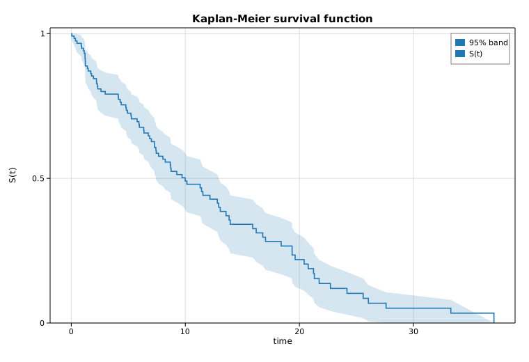
Copula dependence (Clayton)
A copula strips a joint distribution down to its dependence structure: it is the joint law on uniform margins, so all of its content is how the coordinates move together, not where each one lives. The Clayton family models lower-tail dependence — small values of one coordinate strongly pull the other down, while the upper tail is comparatively loose.
This example pins the dependence parameter theta from a target Kendall's tau
with ClaytonCopula::theta_from_tau, evaluates
the closed-form copula density c(u, v) on a grid over the unit square, draws a
deterministic pseudo-random sample by conditional inversion, and recovers the
rank correlations from that sample with
kendalls_tau and
spearmans_rho.
Code
#![allow(unused)]
fn main() {
use solow_copula::{kendalls_tau, spearmans_rho, ClaytonCopula};
use solow_viz::{Color, Colormap, Figure, LineStyle, Marker};

// Pin theta from a target Kendall's tau: tau = theta / (theta + 2).
let target_tau = 0.5;
let theta = ClaytonCopula::theta_from_tau(target_tau);
let cop = ClaytonCopula::new(theta);

// Evaluate the copula density on an n x n grid over the unit square. Row 0 is
// drawn at the TOP of the extent, so v runs from high to low as the row grows.
// The log-density compresses the (0, 0) corner spike into a readable range.
let n = 80usize;
let eps = 1.0 / (n as f64 + 1.0);
let coord = |k: usize| eps + (1.0 - 2.0 * eps) * (k as f64) / ((n - 1) as f64);
let mut grid: Vec<Vec<f64>> = Vec::with_capacity(n);
for r in 0..n {
    let v = coord(n - 1 - r);
    grid.push((0..n).map(|c| cop.pdf(coord(c), v).ln()).collect());
}

// Draw a reproducible sample by conditional inversion (deterministic RNG).
// v = ( u^{-theta} (w^{-theta/(1+theta)} - 1) + 1 )^{-1/theta}, u, w ~ Unif.
let mut rng = common::Rng::new(0xC0FFEE_u64);
let (mut us, mut vs) = (Vec::new(), Vec::new());
for _ in 0..600 {
    let u = rng.uniform().clamp(1e-9, 1.0 - 1e-9);
    let w = rng.uniform().clamp(1e-9, 1.0 - 1e-9);
    let a = w.powf(-theta / (1.0 + theta)) - 1.0;
    let v = (u.powf(-theta) * a + 1.0).powf(-1.0 / theta);
    us.push(u);
    vs.push(v.clamp(1e-9, 1.0 - 1e-9));
}

println!("  sample Kendall's tau : {:.4}  (analytic {:.4})",
         kendalls_tau(&us, &vs), cop.tau());
}
The density grid is rendered as a heatmap with the sample scattered on top and
the u = v diagonal — where Clayton concentrates its mass — drawn as a guide:
#![allow(unused)]
fn main() {
let mut fig = Figure::new(720, 640);
let ax = fig.axes();
ax.set_title("Clayton copula density (tau = 0.5)").set_xlabel("u").set_ylabel("v");
ax.heatmap(&grid, Colormap::Viridis, (0.0, 1.0, 0.0, 1.0), true);
ax.scatter_full(&us, &vs, Color::WHITE, 2.0, Marker::Circle, 0.55, Some("sample"));
ax.line(&[0.0, 1.0], &[0.0, 1.0], Color::RED, 1.5, LineStyle::Dashed,
        Marker::None, 0.9, Some("u = v"));
ax.set_xlim(0.0, 1.0).set_ylim(0.0, 1.0);
fig.save_svg("copula_density.svg").unwrap();
}
Printed output
Clayton copula
  target Kendall's tau : 0.5000
  implied theta        : 2.000000
  analytic tau(theta)  : 0.500000
  density landmarks c(u, v):
    c(0.1, 0.1) = 5.3702
    c(0.5, 0.5) = 1.4810
    c(0.9, 0.9) = 2.1578
    c(0.1, 0.9) = 0.0409
  grid: 80 x 80 over (u, v) in (0.0123, 0.9877)
  log-density range    : [-7.6530, 3.7604]
  sample size          : 600
  sample Kendall's tau : 0.4901  (analytic 0.5000)
  sample Spearman rho  : 0.6694
A target Kendall's tau of 0.5 implies theta = 2, and the analytic
tau(theta) recovers 0.5 exactly. The density landmarks tell the lower-tail
story directly: c(0.1, 0.1) = 5.37 is far heavier than the symmetric upper
corner c(0.9, 0.9) = 2.16, while the off-diagonal c(0.1, 0.9) = 0.04 is
nearly empty. The 600-point sample, drawn with the deterministic SplitMix64
generator, recovers a Kendall's tau of 0.4901 — within sampling error of the
analytic 0.5.
Plot
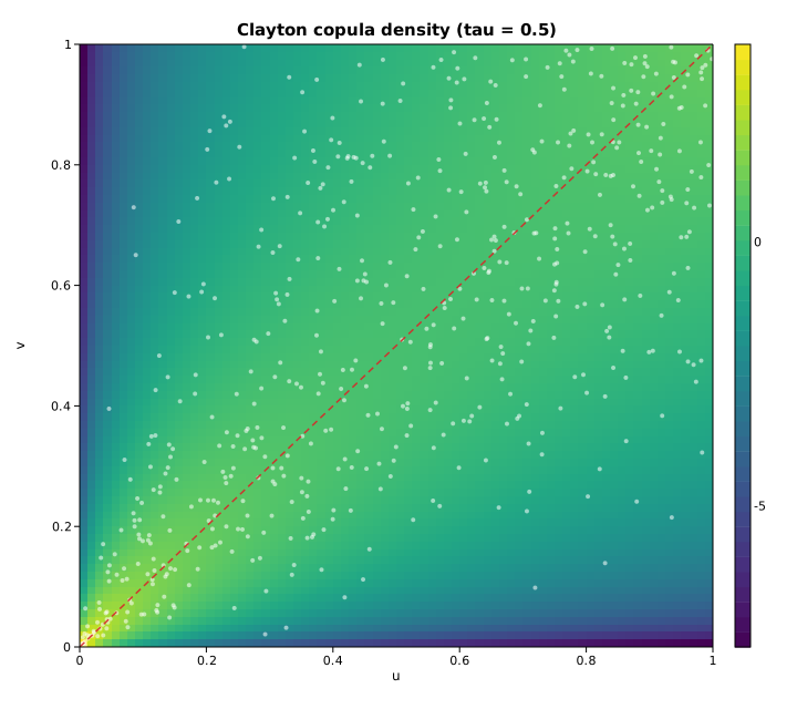
Empirical-likelihood ratio for the mean
Empirical likelihood (EL) turns the nonparametric likelihood of a sample into a
profile statistic. For a hypothesized mean mu, the EL-ratio statistic
-2 log ELR(mu) measures how strongly the data contradict that value; it is
asymptotically chi-squared with one degree of freedom. This example draws a
small reproducible sample, sweeps a grid of hypothesized means with
DescStat::test_mean, and plots the profile
curve against the chi-squared(1) 95% critical value. The two points where the
profile crosses that threshold are the 95% EL confidence interval — which we
cross-check against DescStat::ci_mean.
Code
#![allow(unused)]
fn main() {
use solow_emplike::DescStat;
use solow_viz::{Color, Figure, LegendLoc, LineStyle, Marker};

// Example data: 30 draws from N(5, 2^2) with deterministic pseudo-random noise.
let n = 30usize;
// `data` is built from a seeded SplitMix64 stream, so the run is reproducible.
let sample_mean = data.iter().sum::<f64>() / n as f64;

let d = DescStat::new(&data);

// 95% EL confidence interval for the mean, from the gamma root-finder.
let (ci_lo, ci_hi) = d.ci_mean(0.05);
let crit = 3.841_458_820_694_124_f64; // chi2_ppf(0.95, 1)

// Profile -2 logELR over a grid of hypothesized means.
let (grid_lo, grid_hi) = (sample_mean - 2.2, sample_mean + 2.2);
let steps = 221usize;
let mut mus = Vec::with_capacity(steps);
let mut stats = Vec::with_capacity(steps);
for k in 0..steps {
    let mu = grid_lo + (grid_hi - grid_lo) * (k as f64) / (steps as f64 - 1.0);
    mus.push(mu);
    stats.push(d.test_mean(mu).stat);
}
}
The profile curve is then drawn with the threshold line and the EL confidence band:
#![allow(unused)]
fn main() {
let mut fig = Figure::new(760, 520);
let ax = fig.axes();
ax.set_title("Empirical-likelihood ratio profile for the mean")
    .set_xlabel("hypothesized mean  mu")
    .set_ylabel("-2 log ELR")
    .set_grid(true);

ax.axvspan(ci_lo, ci_hi, Color::BLUE, 0.08); // shade the 95% EL CI
ax.line(&mus, &stats, Color::cycle(0), 2.5, LineStyle::Solid, Marker::None, 1.0,
        Some("-2 log ELR(mu)"));
ax.axhline(crit, Color::RED, LineStyle::Dashed); // chi2(1) 95% threshold
ax.scatter_full(&[ci_lo, ci_hi], &[crit, crit], Color::RED, 5.0, Marker::Circle,
                1.0, Some("95% EL CI endpoints"));
ax.set_ylim(0.0, 12.0);
ax.legend(LegendLoc::UpperRight);
fig.save_svg("emplike_ratio.svg").unwrap();
}
Printed results
Empirical-likelihood ratio for the mean
========================================
nobs              : 30
sample mean       : 4.857548

-2 logELR at sample mean : 0.000000  (p = 1.000000)
-2 logELR at true mean 5 : 0.168374  (p = 0.681561)

chi2(1) 95% threshold    : 3.841459
95% EL CI (ci_mean)      : [4.161524, 5.533040]
-2 logELR at CI endpoints: 3.841459, 3.841459  (should equal threshold)
The statistic vanishes at the sample mean (4.858), as it must, and the true
mean 5 is comfortably inside the interval (p = 0.68). The crucial
cross-check: evaluating -2 log ELR at the two ci_mean endpoints returns
exactly the chi-squared(1) threshold 3.841459, confirming that the curve's
crossings and the closed-form interval [4.162, 5.533] agree.
Plot
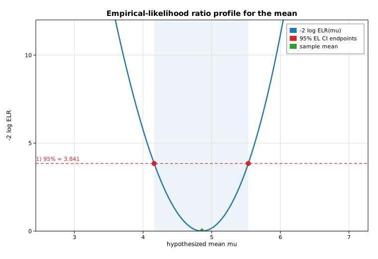
Principal component analysis (PCA)
Principal component analysis finds an orthogonal basis ordered by the amount
of variance each direction captures. It is the standard tool for dimensionality
reduction and exploratory visualization. Solow provides it as
Pca, with an optional standardization
step.
This example generates three clusters in a 4-dimensional feature space, fits PCA on the standardized columns, and produces two classic diagnostics: a scree plot of the per-component variance ratio and a scores scatter of the first two principal components.
Code
#![allow(unused)]
fn main() {
use ndarray::Array2;
use solow_multivariate::Pca;

// Three latent groups in 4-D; 50 points each.
let matrix = Array2::from_shape_vec((n, 4), data).unwrap();

// Fit on standardized columns.
let res = Pca::new(matrix).standardize(true).fit().unwrap();

// Results expose eigenvals, explained_variance_ratio, loadings, and scores.
for i in 0..res.ncomp {
    println!("comp {}: ratio = {:.4}", i + 1, res.explained_variance_ratio[i]);
}
// res.scores is nobs x ncomp; columns 0 and 1 are PC1 and PC2.
}
Printed summary
PCA on 150 observations x 4 variables
  comp    eigenvalue       var ratio      cumulative
     1      272.1529          0.4536          0.4536
     2      180.9883          0.3016          0.7552
     3       95.1618          0.1586          0.9138
     4       51.6970          0.0862          1.0000
The first two components together capture about 76% of the total variance — and, as the scores plot shows, they are exactly the directions that separate the three groups.
Plot
Left: the scree plot (variance ratio per component). Right: the PC1/PC2 scores, colored by the true group label — the three clusters are cleanly separated in the leading two-component subspace.
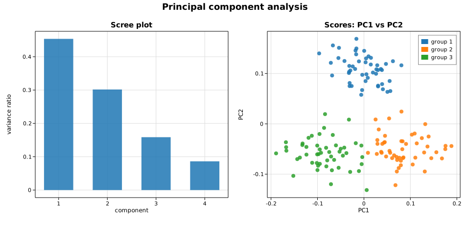
Normal Q-Q plot (probability plot)
A normal quantile-quantile (Q-Q) plot compares the ordered values of a sample
against the quantiles you would expect from a standard normal distribution. If
the sample is approximately normal, the points fall close to a straight line.
This example draws a reproducible standard-normal sample, builds a
ProbPlot from the solow-graphics crate,
prints the computed quantiles and the fitted reference line, and overlays an
ordinary-least-squares reference line on the scatter.
Code
#![allow(unused)]
fn main() {
use solow_graphics::ProbPlot;
use solow_viz::{Color, Figure, LegendLoc, LineStyle, Marker};

// Reproducible sample: 80 draws from N(0, 1) via a deterministic SplitMix64 RNG.
let n = 80usize;
let data: Vec<f64> = (0..n).map(|_| rng.normal()).collect();

// Build the probability plot (standard-normal, Weibull plotting positions).
let pp = ProbPlot::new(&data);
let theo = pp.theoretical_quantiles(); // normal inverse-CDF of the plotting positions
let samp = pp.sample_quantiles();      // the sorted sample
let line = pp.qqline_regression();     // OLS of sample on theoretical quantiles

println!("No. observations:        {}", pp.nobs());
println!("regression (r): slope = {:.4}  intercept = {:.4}", line.slope, line.intercept);
}
The theoretical quantiles (x) and sample quantiles (y) are then scattered, with the OLS reference line drawn across the quantile range:
#![allow(unused)]
fn main() {
let theo_v: Vec<f64> = theo.to_vec();
let samp_v: Vec<f64> = samp.to_vec();
let (lo, hi) = (theo_v[0], theo_v[theo_v.len() - 1]);
let ys_line = [line.slope * lo + line.intercept, line.slope * hi + line.intercept];

let mut fig = Figure::new(760, 520);
let ax = fig.axes();
ax.set_title("Normal Q-Q plot")
    .set_xlabel("Theoretical quantiles")
    .set_ylabel("Sample quantiles")
    .set_grid(true);
ax.scatter_full(&theo_v, &samp_v, Color::cycle(0), 4.0, Marker::Circle, 0.85,
                Some("sample quantiles"));
ax.line(&[lo, hi], &ys_line, Color::RED, 2.5, LineStyle::Solid, Marker::None, 1.0,
        Some("OLS reference line"));
ax.legend(LegendLoc::UpperLeft);
fig.save_svg("graphics_qq.svg").unwrap();
}
Printed output
Normal Q-Q plot (ProbPlot)
==========================
No. observations:        80
Theoretical quantiles:   [-2.2462, ..., 2.2462]
Sample quantiles:        [-2.8317, ..., 2.1851]

Reference lines (y = slope * x + intercept):
  regression (r):  slope = 1.1484   intercept = 0.0601
  standardized (s): slope = 1.0977   intercept = 0.0601
  quartile (q):    slope = 1.1361   intercept = 0.0767
The three reference lines agree closely (slopes near 1.1, intercepts near
0.06), reflecting an approximately normal sample. The regression line r is
the least-squares fit of the sample on the theoretical quantiles; the
standardized line s uses the sample mean and standard deviation; and the
quartile line q passes through the first and third sample quartiles. The
slightly-above-one slope and the low-end sample quantile (-2.83) show this
particular draw has marginally heavier tails than the ideal normal.
Plot
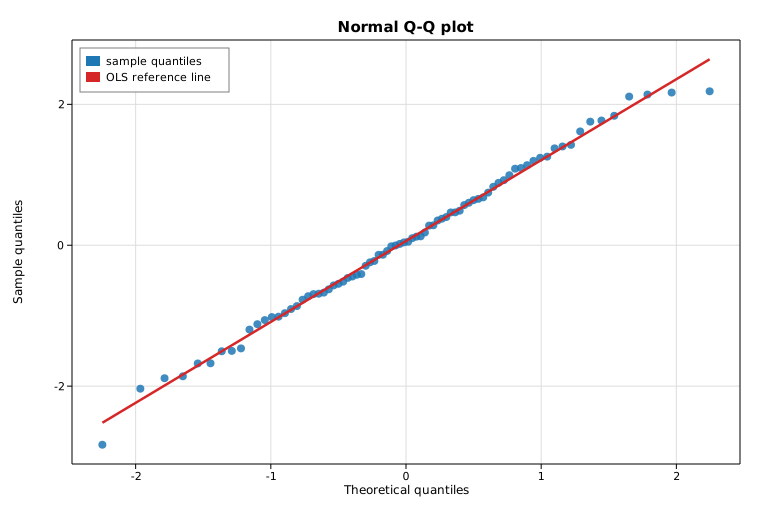
Multiple imputation (MICE)
Multiple imputation handles missing data by filling each gap several times,
analysing every completed data set, and pooling the results so that the extra
uncertainty from the imputation is carried into the final inference. The
solow-impute crate implements the two deterministic pieces of this workflow:
conditional_mean_impute fits a regression on
the observed rows and predicts the conditional mean at the missing rows, and
combine applies Rubin's rules to pool the
per-imputation estimates.
This example builds y = 1.5 + 0.8x + ε, deletes every fifth y value, runs
m = 20 imputations, refits each completed data set by OLS, and pools the slope
with Rubin's rules. The stochastic residual draw that turns the single
conditional mean into a proper imputation is supplied by the gallery's
deterministic RNG, so the whole run is reproducible.
Code
#![allow(unused)] fn main() { use ndarray::{Array1, Array2}; use solow_impute::{combine, conditional_mean_impute}; use solow_regression::LinearModel; // Complete data y = 1.5 + 0.8 x + N(0, 1), x = 0, 1, ..., 39, then delete // every fifth y (MCAR). `observed` / `missing` index the two row blocks. let endog_obs = Array1::from(observed.iter().map(|&i| y_full[i]).collect::<Vec<_>>()); let exog_obs = /* [1, x] design over the observed rows */; let exog_miss = /* [1, x] design over the missing rows */; // One deterministic conditional-mean fit; `scale` is the residual variance. let imp = conditional_mean_impute(endog_obs, exog_obs, &exog_miss).unwrap(); let resid_sd = imp.scale.sqrt(); // m imputations: conditional mean + one residual-scale draw per missing cell, // then refit the completed data set and collect (params, cov_params). let mut params_list: Vec<Array1<f64>> = Vec::new(); let mut cov_list: Vec<Array2<f64>> = Vec::new(); for _ in 0..20 { let mut y = y_full.clone(); for (k, &i) in missing.iter().enumerate() { y[i] = imp.imputed_missing[k] + resid_sd * rng.normal(); } let res = LinearModel::ols(Array1::from(y), design_full.clone()) .unwrap() .fit() .unwrap(); params_list.push(res.params.clone()); cov_list.push(res.cov_params.clone()); } // Pool with Rubin's rules; dfcom is the observed-fit residual df. let pooled = combine(¶ms_list, &cov_list, dfcom).unwrap(); let ci = pooled.conf_int(0.05); }
The pooled slope is then drawn as a point-with-error-bar (its 95% CI) alongside
the observed and imputed (x, y) points and the pooled regression line:
#![allow(unused)]
fn main() {
let slope = pooled.params[1];
let half = (ci[[1, 1]] - ci[[1, 0]]) / 2.0;
ax.scatter_full(&x_obs, &y_obs, Color::BLUE, 5.0, Marker::Circle, 0.85, Some("observed"));
ax.scatter_full(&x_mis, &imputed_first, Color::RED, 7.0, Marker::Diamond, 0.95, Some("imputed (draw 1)"));
ax.errorbar(&[x_hi + 0.5], &[slope], &[half], Color::GREEN, Some("pooled slope b1 (95% CI)"));
fig.save_svg("mice_convergence.svg").unwrap();
}
Printed results
conditional-mean imputation
  fit on 32 observed rows: y_hat = 1.3950 + 0.8057 x   (residual sd = 0.9751)
  8 missing rows imputed at their conditional means:
    row  0: x =  0.0   y_imputed =  1.3950
    row  5: x =  5.0   y_imputed =  5.4236
    row 10: x = 10.0   y_imputed =  9.4523
    row 15: x = 15.0   y_imputed = 13.4809
    row 20: x = 20.0   y_imputed = 17.5096
    row 25: x = 25.0   y_imputed = 21.5382
    row 30: x = 30.0   y_imputed = 25.5668
    row 35: x = 35.0   y_imputed = 29.5955

pooled estimate over m = 20 imputations (Rubin's rules)
  param        coef    std err        fmi         df         95% conf. int.
  const      1.4215     0.3227     0.1245      24.19   [  0.7557,   2.0874]
  x          0.8050     0.0145     0.1517      23.23   [  0.7751,   0.8349]
The pooled slope 0.805 recovers the true 0.8 and the intercept 1.42 is
close to 1.5; the 95% interval for the slope ([0.775, 0.835]) covers the
truth. The fraction of missing information (fmi ≈ 0.12–0.15) reflects the
8-of-40 deleted y values, and the Barnard–Rubin degrees of freedom (≈ 23–24)
are well below the complete-data df, the price multiple imputation pays for the
gaps.
Plot
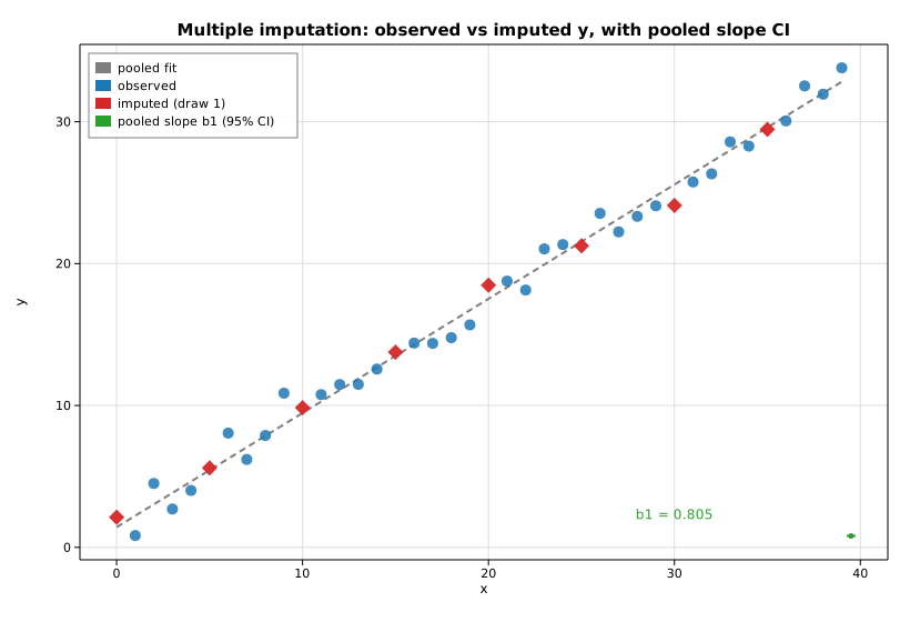
Bayesian mixed GLM (variational Bayes)
A Bayesian generalized linear mixed model adds Gaussian random effects to a GLM. Here we fit a binomial (logit-link) model with a per-group random intercept,
logit P(yᵢ = 1) = b₀ + b₁ xᵢ + u_group(i), u_g ~ N(0, σ_u²),
using BayesMixedGlm::fit_vb, which maximizes the
evidence lower bound (ELBO) of a mean-field Gaussian variational posterior. This
is deterministic variational Bayes, not MCMC: the fit returns a posterior
mean and posterior standard deviation for every parameter (an approximate
Gaussian posterior), so we summarize the fixed effects as point estimates with
±2 posterior-sd credible bands rather than drawing samples.
The data is synthesized from the generative model above with the gallery's deterministic SplitMix64 RNG (8 groups × 12 observations = 96 rows), so the run is fully reproducible.
Code
#![allow(unused)]
fn main() {
use ndarray::{Array1, Array2};
use solow_bayes::{BayesMixedGlm, Family};
use solow_viz::{Color, Figure, LegendLoc, LineStyle};

// Generative model: logit P(y=1) = -0.4 + 1.3 x + u_g,  u_g ~ N(0, 0.8²).
let (n_groups, per) = (8usize, 12usize);
let n = n_groups * per;
let (true_b0, true_b1, true_sigma_u) = (-0.4_f64, 1.3, 0.8);

let mut rng = common::Rng::new(20240618);
let group_u: Vec<f64> = (0..n_groups).map(|_| true_sigma_u * rng.normal()).collect();

// Fixed-effects design [1, x]; random-effects design = one indicator column
// per group (a random intercept). `ident` ties every group column to a single
// variance component (one shared log-sd parameter).
let mut exog = Array2::<f64>::zeros((n, 2));
let mut exog_vc = Array2::<f64>::zeros((n, n_groups));
let mut endog = Array1::<f64>::zeros(n);
for i in 0..n {
    let g = i / per;
    let xi = -1.5 + 3.0 * (i % per) as f64 / (per as f64 - 1.0);
    let eta = true_b0 + true_b1 * xi + group_u[g];
    let p = 1.0 / (1.0 + (-eta).exp());
    exog[[i, 0]] = 1.0;
    exog[[i, 1]] = xi;
    exog_vc[[i, g]] = 1.0;
    endog[i] = rng.bernoulli(p);
}
let ident = vec![0usize; n_groups];

// Fit by variational Bayes. vcp_p / fe_p are the prior sds for the
// variance-component log-sd and the fixed effects.
let model =
    BayesMixedGlm::new(Family::Binomial, endog, exog, exog_vc, ident, 1.0, 4.0).unwrap();
let res = model.fit_vb(None, None, 100_000, 1e-6).unwrap();

// res.fe_mean / res.fe_sd  -> fixed-effect posterior mean & sd
// res.vcp_mean             -> log-sd of the random intercept (exp -> sigma_u)
// res.vc_mean / res.vc_sd  -> per-group random-intercept posteriors
// res.elbo                 -> maximized ELBO (the variational log-likelihood)
}
The fixed-effect posteriors are then plotted as points with ±2 posterior-sd credible bands, with the data-generating truth marked for reference:
#![allow(unused)]
fn main() {
let xs = [0.0_f64, 1.0];
let means = [res.fe_mean[0], res.fe_mean[1]];
let err2 = [2.0 * res.fe_sd[0], 2.0 * res.fe_sd[1]];
let truth = [true_b0, true_b1];

let mut fig = Figure::new(760, 520);
let ax = fig.axes();
ax.set_title("Bayesian mixed GLM (VB): fixed-effect posteriors")
    .set_xlabel("fixed effect").set_ylabel("coefficient").set_grid(true);
ax.set_xlim(-0.6, 1.6);
ax.axhline(0.0, Color::GRAY, LineStyle::Dotted);
ax.errorbar(&xs, &means, &err2, Color::cycle(0), Some("posterior mean +/- 2 sd"));
ax.scatter_full(&xs, &truth, Color::RED, 6.0, solow_viz::Marker::Diamond, 1.0, Some("true value"));
ax.legend(LegendLoc::UpperLeft);
fig.save_svg("bayes_posterior.svg").unwrap();
}
Printed results
Bayesian mixed GLM (binomial / logit) by variational Bayes
  observations: 96   groups: 8   per group: 12
  converged: true   iters: 23   |grad|: 2.764e-7   ELBO: -63.481683

Fixed effects (approximate Gaussian posterior):
  name               post. mean     post. sd    post. mean +/- 2 sd
  intercept (b0)       -0.80040      0.24613   -1.29267 .. -0.30814
  slope (b1)            1.00540      0.27225    0.46090 ..  1.54991

Variance component (group random intercept, log-sd):
  vcp posterior mean: -0.02104   posterior sd: 0.24284
  implied sigma_u = exp(vcp_mean): 0.97918   (true 0.800)

Random intercept posterior means by group (vc_mean):
  group  0: post. mean  0.24616  post. sd 0.53770  (true u  0.48418)
  group  1: post. mean -1.05301  post. sd 0.60813  (true u -1.18688)
  group  2: post. mean -0.36203  post. sd 0.56185  (true u -0.80476)
  group  3: post. mean -0.36203  post. sd 0.56185  (true u -0.83760)
  group  4: post. mean -0.36203  post. sd 0.56185  (true u -1.28414)
  group  5: post. mean  0.81912  post. sd 0.53053  (true u  0.23701)
  group  6: post. mean  1.39322  post. sd 0.53873  (true u  0.90634)
  group  7: post. mean -0.36203  post. sd 0.56185  (true u -1.05832)
The 95%-style credible band for the slope (0.461 … 1.550) comfortably covers
the true 1.3, and the band for the intercept (-1.293 … -0.308) covers the
true -0.4; with only 96 binary observations the variational posterior is
appropriately wide. The recovered group-intercept sd, exp(vcp_mean) ≈ 0.979,
is in the right neighborhood of the true 0.8 (a single small sample identifies
a scale parameter only loosely).
Two honest caveats worth noting. First, several groups (2, 3, 4, 7) land on the
identical posterior mean -0.36203: with the same within-group x grid these
groups happened to draw the same 0/1 outcome pattern, so they share sufficient
statistics and the posterior cannot distinguish them — the random-effect means
shrink them all toward the common value. Second, variational Bayes is known to
understate posterior uncertainty relative to full MCMC, so these bands should
be read as the variational approximation's credible intervals, not as exact
posterior intervals.
Plot
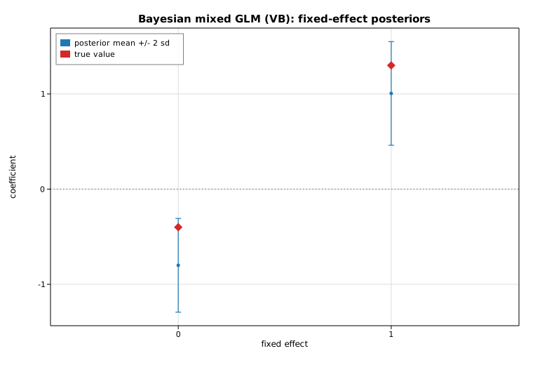
Optimizer convergence
The optimizers in solow-optimize minimize an
objective by driving its gradient to zero. This example runs two of them on
standard test functions and plots how fast each one converges:
- the Rosenbrock banana, minimized with
minimize_bfgs(gradient only — supplied here by central finite differences viaapprox_fprime); - a convex quadratic, minimized with
newton_stationary(analytic gradient and Hessian).
Neither solver exposes a per-iteration trace, so the convergence curve is built
honestly: each solver is re-run from the same start with an increasing iteration
cap k = 0, 1, 2, …, and the final gradient norm reported by the returned
OptimizeResult is recorded at each cap. On a log y-scale the convergence
rate becomes a slope — BFGS descends steadily, while Newton lands on the
quadratic's minimum in a single step.
Code
#![allow(unused)]
fn main() {
use ndarray::{array, Array1, Array2};
use solow_optimize::{approx_fprime, minimize_bfgs, newton_stationary};
use solow_viz::{Color, Figure, LegendLoc, LineStyle, Marker, Scale};

// Rosenbrock f(x) = (1 - x0)^2 + 100 (x1 - x0^2)^2, global min 0 at (1, 1).
fn rosenbrock(x: &Array1<f64>) -> f64 {
    (1.0 - x[0]).powi(2) + 100.0 * (x[1] - x[0] * x[0]).powi(2)
}

// Curve 1: BFGS on Rosenbrock, gradient from finite differences.
let start_rb = array![-1.2, 1.0];
let gtol = 1e-10;
let mut rb_iter: Vec<f64> = Vec::new();
let mut rb_gnorm: Vec<f64> = Vec::new();
for k in 0..=40 {
    let g = |x: &Array1<f64>| approx_fprime(x, rosenbrock);
    let r = minimize_bfgs(&start_rb, rosenbrock, g, k, gtol).unwrap();
    rb_iter.push(r.iters as f64);
    rb_gnorm.push(r.grad_norm.max(1e-16)); // floor for the log axis
}

// Curve 2: Newton on a convex quadratic, analytic g and H.
// f(x) = (x0 - 3)^2 + 2 (x1 + 1)^2, min 0 at (3, -1).
let fgh = |x: &Array1<f64>| {
    let f = (x[0] - 3.0).powi(2) + 2.0 * (x[1] + 1.0).powi(2);
    let g = array![2.0 * (x[0] - 3.0), 4.0 * (x[1] + 1.0)];
    let h: Array2<f64> = array![[2.0, 0.0], [0.0, 4.0]];
    (f, g, h)
};
let start_q = array![0.0, 0.0];
let mut q_iter: Vec<f64> = Vec::new();
let mut q_gnorm: Vec<f64> = Vec::new();
for k in 0..=6 {
    let r = newton_stationary(&start_q, fgh, k, gtol).unwrap();
    q_iter.push(r.iters as f64);
    q_gnorm.push(r.grad_norm.max(1e-16));
}
}
The two convergence curves are then drawn on a shared log y-scale:
#![allow(unused)]
fn main() {
let mut fig = Figure::new(760, 520);
let ax = fig.axes();
ax.set_title("Optimizer convergence: gradient norm vs iteration")
    .set_xlabel("iteration")
    .set_ylabel("gradient norm  (log scale)")
    .set_yscale(Scale::Log)
    .set_grid(true);
ax.line(&rb_iter, &rb_gnorm, Color::cycle(0), 2.0, LineStyle::Solid,
        Marker::Circle, 0.9, Some("BFGS, Rosenbrock"));
ax.line(&q_iter, &q_gnorm, Color::RED, 2.0, LineStyle::Dashed,
        Marker::Square, 0.9, Some("Newton, quadratic"));
ax.legend(LegendLoc::UpperRight);
fig.save_svg("optim_convergence.svg").unwrap();
}
Printed results
Optimizer convergence
=====================================================
BFGS on Rosenbrock  (start = [-1.2, 1.0])
  x* = [1.000000, 1.000000]
  f(x*)      = 6.410136e-19
  grad_norm  = 1.143454e-11
  iters      = 36
  converged  = true
-----------------------------------------------------
Newton on quadratic (start = [0.0, 0.0])
  x* = [3.000000, -1.000000]
  f(x*)      = 0.000000e0
  grad_norm  = 0.000000e0
  iters      = 1
  converged  = true
-----------------------------------------------------
Gradient norm vs iteration cap (BFGS / Rosenbrock):
  cap  0 -> iters  0  grad_norm = 2.3287e2
  cap  5 -> iters  5  grad_norm = 4.0462e0
  cap 10 -> iters 10  grad_norm = 6.8753e0
  cap 15 -> iters 15  grad_norm = 1.5209e0
  cap 20 -> iters 20  grad_norm = 5.8425e-1
  cap 25 -> iters 25  grad_norm = 1.6586e0
  cap 30 -> iters 30  grad_norm = 1.9769e-1
  cap 35 -> iters 35  grad_norm = 9.5186e-10
  cap 40 -> iters 36  grad_norm = 1.1435e-11
Newton reaches the quadratic's minimum (3, -1) exactly in one step, since the
Newton update is exact for a quadratic. BFGS needs 36 iterations to thread the
Rosenbrock valley but ends at (1, 1) with a gradient norm of 1.14e-11 — the
non-monotone early plateau (the gradient norm even rises around iteration 10 as
the iterate rounds the bend of the banana) gives way to a sharp final descent
once it reaches the smooth basin near the optimum.
Plot
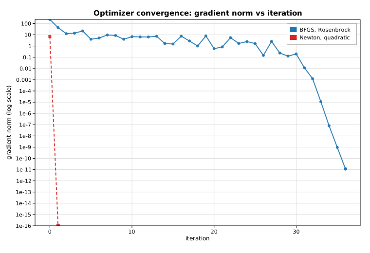
The formula interface
The formula API (solow-fit) is the one-call bridge from an R/patsy-style
formula string plus a named DataFrame to a fully fitted model whose
coefficients are already labeled with the design-matrix column names. It is
the from-scratch equivalent of the reference library's from_formula
constructors: no hand-assembled design matrix, no manually threaded column
names.
This example fits
y ~ x1 + x2 + C(group)
mixing two numeric predictors with a three-level categorical factor (expanded into treatment-coded dummy columns), then shows that a Poisson GLM is just as easy to fit from a formula.
Code
#![allow(unused)]
fn main() {
use solow_fit::{ols, poisson, DataFrame};

let mut df = DataFrame::new();
df.add_numeric("y", y);
df.add_numeric("x1", x1);
df.add_numeric("x2", x2);
df.add_categorical("group", g);          // levels "A", "B", "C"

// Fit OLS straight from the formula; coefficients come back labeled.
let fit = ols("y ~ x1 + x2 + C(group)", &df).unwrap();
println!("Design columns: {:?}", fit.names());
println!("{}", fit.summary());

// The same ergonomics for a Poisson GLM.
let pfit = poisson("count ~ x1", &dfp).unwrap();
println!("{}", pfit.summary());
}
C(group) expands to two treatment-coded dummies ([T.B], [T.C]) relative to
the reference level A, and the intercept is added automatically.
Printed summary
OLS from formula: y ~ x1 + x2 + C(group)
Design columns: ["Intercept", "C(group)[T.B]", "C(group)[T.C]", "x1", "x2"]

      Regression Results
==============================
Statistic                Value
------------------------------
Model:                     OLS
No. Observations:           90
Df Model:                    4
Df Residuals:               85
R-squared:               0.947
Adj. R-squared:          0.944
F-statistic:             379.1
Prob (F-statistic):  2.670e-53
Log-Likelihood:        -69.957
AIC:                    149.91
BIC:                    162.41
==============================

==============================================================
                 coef  std err        t  P>|t|  [0.025  0.975]
--------------------------------------------------------------
Intercept      0.7385   0.1335    5.532  0.000   0.473   1.004
C(group)[T.B]   2.663   0.1412   18.856  0.000   2.382   2.943
C(group)[T.C]  -1.451   0.1399  -10.371  0.000  -1.730  -1.173
x1             0.8635  0.03877   22.272  0.000   0.786   0.941
x2             -1.222  0.05772  -21.171  0.000  -1.337  -1.107
==============================================================
The estimated coefficients recover the true generating values: slopes of
+0.8 on x1 and −1.2 on x2, and group offsets of +2.5 (B) and −1.5
(C) relative to A. The Poisson model fit from count ~ x1 is printed below it
in the program's output.
Plot
Observed response against the formula model's fitted values, with the y = ŷ
reference diagonal — points hug the line because the model explains ~95% of the
variance.
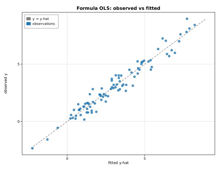
API reference
This user guide is the narrative documentation — concepts, model definitions,
worked examples, and plots. The complete, per-function API reference (every
public type, method, field, and free function, with signatures and doc
comments) is the generated rustdoc.
-
Online: once a crate is published, its reference lives at
https://docs.rs/<crate>— for exampledocs.rs/solow-regression. The docs.rs build is automatic; every release is rendered there. -
Locally: build it from the source tree with
cargo doc --no-deps --workspace --openThis produces the same reference under
target/doc/and opens it in your browser. The whole workspace documents with zero warnings.
Each guide page ends with a Module reference table listing that area's key public items; the links below take you to the full rustdoc for the crate behind each area.
Crates by area
Foundational crates
These underpin everything above and are usually used indirectly:
| Crate | Role | API reference |
|---|---|---|
solow | Umbrella crate re-exporting the stack | docs.rs |
solow-core | Shared error type and data tools | docs.rs |
solow-linalg | From-scratch linear algebra (SVD, eigh, QR, Cholesky) | docs.rs |
solow-viz | Dependency-light SVG plotting backend | docs.rs |
Using Solow from Python
Solow ships PyO3 bindings (solow-py) that compile to a native CPython
extension module named solow. The bindings marshal NumPy float64 arrays into
Solow's estimators and return NumPy arrays and Python floats. They are verified
to reproduce the reference outputs to roughly 1e-12 from Python.
The solow-py crate is its own standalone Cargo workspace (excluded from the
umbrella workspace) so it can be built independently with the
extension-module feature.
The Python API
Every model takes endog (a 1-D float64 array) and exog (a 2-D float64
array). As with the reference stack, you supply any intercept column
yourself — no constant is added automatically.
import numpy as np
import solow

# A design matrix with an explicit constant column.
n = 50
rng = np.random.default_rng(0)
x = rng.standard_normal(n)
X = np.column_stack([np.ones(n), x])           # [const, x]
y = 1.0 + 2.0 * x + 0.1 * rng.standard_normal(n)

# Ordinary least squares.
res = solow.OLS(y, X).fit()
print(res.params)        # ndarray of coefficients
print(res.bse)           # standard errors
print(res.tvalues)       # t-statistics
print(res.pvalues)       # p-values
print(res.conf_int)      # (k, 2) ndarray, 95% (alpha = 0.05)
print(res.rsquared, res.rsquared_adj, res.fvalue, res.f_pvalue)
print(res.aic, res.bic, res.llf, res.nobs, res.df_model, res.df_resid)
print(res.fittedvalues, res.resid)
solow.WLS(y, X, weights) and solow.GLS(y, X, sigma) cover weighted and
generalized least squares; the weights are per-observation (positive,
proportional to the inverse error variance) and sigma is the (n, n) SPD
error covariance.
Robust (sandwich) standard errors
For an OLS fit, request heteroskedasticity- or autocorrelation-consistent standard errors without re-fitting:
import solow

res = solow.OLS(y, X).fit()
res.bse_robust("HC1")                      # HC0 | HC1 | HC2 | HC3
res.bse_robust("HAC", maxlags=4)           # Newey-West (use_correction=False)
res.bse_robust("cluster", groups=g)        # g: int64 array (use_correction=True)
res.cov_params_robust("HC3")               # the full (k, k) covariance matrix
The defaults match the reference: no small-sample correction for HAC, the
G/(G-1) * (n-1)/(n-k) correction for clusters. Pass use_correction=... to
override.
Generalized linear models
family is one of "gaussian", "binomial", "poisson", "gamma", or
"inversegaussian". link is optional and defaults to the family's canonical
link.
import solow

res = solow.GLM(y, X, family="poisson").fit()
res = solow.GLM(y, X, family="binomial", link="logit").fit()

print(res.params, res.bse, res.deviance, res.llf, res.aic, res.converged)
Discrete maximum-likelihood models
import solow

res = solow.Logit(y, X).fit()
res = solow.Probit(y, X).fit()
res = solow.Poisson(y, X).fit()

print(res.params, res.bse, res.tvalues, res.pvalues)
print(res.llf, res.aic, res.bic, res.converged)
Time series
import solow

# Autoregression; trend is one of "n" | "c" | "t" | "ct" | "ctt".
res = solow.AutoReg(x, lags=2, trend="c").fit()
print(res.params, res.bse, res.tvalues, res.pvalues)
print(res.sigma2, res.llf, res.aic, res.bic, res.hqic)

# Autocorrelation diagnostics.
a = solow.acf(x, nlags=10)                 # length nlags+1, a[0] == 1
p = solow.pacf(x, nlags=10, method="yw")   # method = "yw" | "ols"
Invalid shapes or non-convergence raise ValueError.
Building the extension
maturin is the usual tool, but it is optional — a plain Cargo build works.
From the crates/solow-py directory (it is a standalone workspace):
PYO3_PYTHON=$(which python3) cargo build --release
The output is a C dynamic library:
- macOS:
target/release/libsolow.dylib - Linux:
target/release/libsolow.so
Copy it next to your code with an extension suffix CPython recognizes. Because
the crate is built with the abi3-py39 feature, a single .abi3.so binary is
compatible with CPython 3.9 and newer:
mkdir -p pytest_dir
cp target/release/libsolow.dylib pytest_dir/solow.abi3.so   # macOS
PYTHONPATH=pytest_dir python3 -c "import solow; print(solow.__version__)"
On macOS the crate's bundled .cargo/config.toml passes
-undefined dynamic_lookup to the linker so the extension imports cleanly;
building through maturin would arrange this automatically.
Verification from Python
The bindings exist not only for convenience but as an independent check: the
solow-py test suite fits each model in both Solow and the authoritative
reference on the same data and asserts agreement to about 1e-12. If you are
migrating Python code, you can swap import solow in for the reference import
on the supported models and expect the same numbers.
Verification & methodology
Solow's central claim is not "these look like reasonable numbers" but "these are the same numbers an authoritative reference produces." This chapter explains how that claim is enforced, the naming discipline behind it, and how to add a new model with its own verification fixture.
The golden-fixture harness
Verification is built on golden fixtures: frozen numerical outputs captured
once from an authoritative Python reference and committed to the repository as
JSON. The Rust test suites read those committed files and assert that Solow
reproduces every value to a tight tolerance. Crucially, the tests need no
Python at test time — cargo test runs against the frozen numbers.
The flow has three pieces:
-
Generators —
tools/reference/gen_*.pyscripts call the reference (andnumpy/scipyfor the linear-algebra and distribution fixtures) and dump results totests/fixtures/*.json. There is roughly one generator per area (gen_models.py,gen_glm.py,gen_discrete.py,gen_duration.py,gen_multivariate.py, …), often with_extcompanions for extended coverage. -
Fixtures —
tests/fixtures/*.jsonhold the committed golden values: inputs, the reference's parameter estimates, standard errors, and the other reported statistics. -
Rust tests — each crate has a
tests/reference*.rsthat loads its fixture and compares Solow's output element-by-element.
tools/reference/gen_models.py  ──►  tests/fixtures/models.json  ──►  crates/solow-regression/tests/reference.rs
        (run once, by a human)            (committed JSON)                 (runs on every `cargo test`)
Tolerances
Agreement is asserted to a tolerance appropriate to each computation:
| Area | Tolerance |
|---|---|
| Most quantities (regression, distributions, tests) | 1e-8 |
| Maximum-likelihood / variational-Bayes estimates | 1e-6 |
| The formula engine (design matrices) | 1e-12 |
| The Python bindings vs. the Rust results | ~1e-12 |
The MLE tolerance is looser only because two independent optimizers converging
to the same optimum agree to optimizer precision, not to the last bit; the
underlying closed-form quantities still match to 1e-8 or better.
Regenerating fixtures
The numpy/scipy-based fixtures regenerate directly:
python3 tools/reference/gen_linalg.py
python3 tools/reference/gen_distributions.py
The modeling fixtures load the reference statistics package indirectly, by a module name supplied through an environment variable, so the repository never hard-codes that package's name:
SOLOW_REFERENCE=<reference-import-name> python3 tools/reference/gen_models.py
The naming discipline
This indirection is deliberate and is enforced as a project rule: the name of
the source statistics package never appears in the Solow source tree. The
reference is loaded through SOLOW_REFERENCE at fixture-generation time and is
referred to in prose only as "the reference" or "an authoritative reference."
Comparison against the broader scientific-Python ecosystem (numpy, scipy,
matplotlib, patsy) is named freely; those are general tools, not the
specific package Solow re-implements.
The reason is that Solow is an independent, from-scratch re-implementation, not a wrapper or a fork. Keeping the source name out of the tree keeps that boundary clean while still letting the test suite prove numerical equivalence.
Adding a model and its fixture
To add a new estimator with verification, follow the same pattern every existing crate uses:
-
Implement the model in its crate (e.g.
crates/solow-yourarea/src/), exposing a results struct with the standard fields (params,bse,tvalues,pvalues, information criteria, …). -
Write a generator
tools/reference/gen_yourarea.pythat fits the same model in the reference on a fixed input and writes the inputs plus the reference outputs totests/fixtures/yourarea.json. Load the reference via theSOLOW_REFERENCEenvironment variable — never import it by name. -
Generate the fixture once and commit the JSON:
SOLOW_REFERENCE=<reference-import-name> python3 tools/reference/gen_yourarea.py -
Add a Rust test
crates/solow-yourarea/tests/reference.rsthat reads the fixture, fits the model with Solow on the same input, and asserts each value agrees within the appropriate tolerance (use theapproxcrate'sassert_abs_diff_eq!). -
Run it offline:
cargo test -p solow-yourareanow verifies against the frozen numbers with no Python in the loop.
Because the fixtures are committed, contributors and CI verify correctness without any reference installation; only regenerating a fixture (when the input or the reference version changes) needs Python.
Verifying the snippets in this book
Every Rust snippet printed in this guide is itself compile-checked against the
real crate APIs. The examples are pasted into a scratch crate that depends on the
Solow crates by path and built with cargo build; a signature mismatch fails the
build. This keeps the documentation honest as the API evolves.
Crate reference
Solow is a Cargo workspace of 54 focused crates. Depend on the ones you
need, or pull in the umbrella solow crate to re-export the full public API.
This page lists the workspace.
Foundation
| Crate | Purpose |
|---|---|
solow-core | Error types, numeric aliases, shared data-handling tools |
solow-linalg | Pure-Rust linear algebra (SVD, eigh, Cholesky, QR, LU, pinv) |
solow-distributions | Special functions, distributions, ECDF, GEV, GPD |
solow-optimize | Newton / BFGS optimizers and numerical differentiation |
Classical statistical models
| Crate | Models |
|---|---|
solow-regression | OLS, WLS, GLS, GLSAR, penalised (Ridge, Lasso, ElasticNet), CV variants, quantile, rolling/recursive, LARS, LassoLars, LassoLarsIC, OMP, HuberRegressor, BayesianRidge, ARDRegression, RANSACRegressor, TheilSenRegressor, MultiTaskLasso/ElasticNet, SGD (regressor + classifier), Perceptron, PassiveAggressive*, RidgeClassifier(CV), Dummy*, KernelRidge, sliced inverse regression, robust covariances |
solow-glm | Generalized linear models (families, links, IRLS) + Tweedie, PoissonRegressor, GammaRegressor, TweedieRegressor |
solow-discrete | Logit, Probit, Poisson, MNLogit, NegativeBinomial, GeneralizedPoisson, OrderedModel, ZeroInflatedPoisson, ConditionalLogit/Poisson, TruncatedLFPoisson, HurdleCountModel, LogisticRegressionCV |
solow-robust | Robust linear models (M-estimation) |
solow-nonparametric | Nonparametric smoothers (lowess, KDE, kernel regression) |
solow-multivariate | PCA, factor analysis and rotation, MANOVA, canonical correlation |
solow-duration | Survival analysis (Kaplan-Meier, Cox PH, log-rank) |
solow-mixed | Linear mixed-effects models (REML) |
solow-gee | Generalized estimating equations (incl. nominal/ordinal) |
solow-gam | Generalized additive models (penalized splines) |
solow-impute | MICE combine + SimpleImputer, KnnImputer, IterativeImputer |
solow-regime | Regime-switching models (Markov switching) |
solow-othermod | Beta regression |
solow-copula | Copulas (Archimedean and elliptical) |
solow-bayes | Bayesian mixed GLM (variational Bayes) |
solow-emplike | Empirical-likelihood inference |
Time series
| Crate | Contents |
|---|---|
solow-tsa | acf/pacf, ADF, KPSS, coint, Granger, AutoReg, ARMA, STL, seasonal_decompose, Holt-Winters, HP/BK/CF filters, zivot_andrews, range_unit_root, breakvar heteroskedasticity, GARCH(1,1), change-point detection (CUSUM, PELT, Binary Segmentation), EWMA control chart |
solow-statespace | Kalman filter/smoother, SARIMAX, unobserved components, dynamic factor |
solow-var | VAR, SVAR, VECM / Johansen |
Statistics, formulas, and presentation
| Crate | Purpose |
|---|---|
solow-stats | ANOVA, Tukey HSD, ARCH, RESET, robust sandwich covariances (HC0-3, HAC, cluster), VIF, mediation, Oaxaca, power, proportion, rates, inter-rater (Cohen's / Fleiss' κ), influence, distance correlation, TOST equivalence, contingency, Pearson / Spearman / Kendall correlations, Mann-Whitney U, Kruskal-Wallis, McNemar, χ² contingency, Levene / Bartlett / Fligner variance tests, Shapiro-Wilk, Anderson-Darling, Kolmogorov-Smirnov, Wald-Wolfowitz runs, meta-analysis (fixed + DerSimonian-Laird random) |
solow-formula | R/patsy-style formula interface (design matrices) |
solow-summary | Labeled results and summary tables |
solow-graphics | Statistical graphics (qqplot, plot_acf, influence) |
solow-viz | General-purpose data-visualization backend (SVG); ROC / PR / reliability / residuals diagnostics |
Model evaluation & resampling
| Crate | Purpose |
|---|---|
solow-metrics | Regression / classification / forecast losses, calibration + post-hoc calibrators (Platt, isotonic, temperature), conformal (split, jackknife+), Diebold-Mariano and Giacomini-White, Friedman / Nemenyi / Wilcoxon, WAIC / PSIS-LOO, permutation importance, partial dependence, ALE, pairwise distances + kernels (RBF / linear / polynomial / sigmoid / laplacian / cosine / χ²), cluster evaluation (silhouette, ARI, MI variants, homogeneity / completeness / v-measure, Fowlkes-Mallows, Calinski-Harabasz, Davies-Bouldin), effect sizes (Cohen's d, Hedges' g, Glass's Δ, η², ω², Cliff's δ, Cramér's V), classification_report |
solow-cv | K-fold, stratified, walk-forward, leave-one-out, leave-p-out, shuffle-split, group-aware, purged / combinatorial-purged K-fold; repeated K-fold / stratified K-fold; stratified & group shuffle split; cross_val_score scoring; learning_curve, validation_curve, permutation_test_score; bootstrap CIs (percentile, basic, BCa); moving / circular / stationary block bootstrap for time series; optional rayon-parallel fold evaluation |
Machine learning
| Crate | Purpose |
|---|---|
solow-preprocessing | 18 preprocessors: Standard/MinMax/MaxAbs/Robust scalers, Normalizer, LabelEncoder, OrdinalEncoder, OneHotEncoder, PolynomialFeatures, KBinsDiscretizer (uniform / quantile / KMeans), PowerTransformer (Yeo-Johnson / Box-Cox), QuantileTransformer, Binarizer, LabelBinarizer, MultiLabelBinarizer, FunctionTransformer, SplineTransformer, TargetEncoder |
solow-cluster | 11 algorithms: KMeans (+K-means++), MiniBatchKMeans, BisectingKMeans, DBSCAN, HDBSCAN, OPTICS, MeanShift, AffinityPropagation, SpectralClustering, AgglomerativeClustering (single/complete/average/Ward), Birch + 2 mixtures: GaussianMixture, BayesianGaussianMixture |
solow-neighbors | KdTree, BallTree, KNeighborsClassifier / KNeighborsRegressor (uniform / distance weights), RadiusNeighborsClassifier / RadiusNeighborsRegressor, NearestCentroid, LocalOutlierFactor, KernelDensity (multivariate) |
solow-tree | DecisionTreeClassifier, DecisionTreeRegressor, ExtraTreeClassifier, ExtraTreeRegressor |
solow-ensemble | RandomForest*, ExtraTrees*, GradientBoosting*, HistGradientBoosting*, Bagging*, AdaBoost (classifier + regressor), Voting (classifier + regressor), Stacking (classifier + regressor), IsolationForest |
solow-naive-bayes | GaussianNB, MultinomialNB, BernoulliNB, ComplementNB, CategoricalNB |
solow-discriminant | LinearDiscriminantAnalysis, QuadraticDiscriminantAnalysis |
solow-feature-selection | SelectKBest, RFE, VarianceThreshold, SelectPercentile, SelectFpr, SelectFdr, SelectFwe, SequentialFeatureSelector |
solow-pipeline | Pipeline, FeatureUnion, ColumnTransformer, TransformedTargetRegressor, GridSearchCV, RandomizedSearchCV, HalvingGridSearchCV, HalvingRandomSearchCV |
solow-svm | LinearSVC, LinearSVR, SVC, SVR, NuSVC, NuSVR, OneClassSVM (kernels: linear / RBF / polynomial / sigmoid) |
solow-neural | MLPClassifier, MLPRegressor (SGD + Adam), BernoulliRBM |
solow-manifold | Isomap, LocallyLinearEmbedding, MDS, SpectralEmbedding, t-SNE |
solow-decomposition | Pca, KernelPca, FastIca, Nmf, MiniBatchNmf, TruncatedSVD, IncrementalPCA, SparsePCA, DictionaryLearning, MiniBatchDictionaryLearning, LatentDirichletAllocation, GaussianRandomProjection, SparseRandomProjection |
solow-text | CountVectorizer, TfidfVectorizer, HashingVectorizer, FeatureHasher, DictVectorizer |
solow-covariance | EmpiricalCovariance, ShrunkCovariance, LedoitWolf, Oas, MinCovDet, GraphicalLasso, EllipticEnvelope |
solow-cross-decomposition | PLSRegression, PLSCanonical, PLSSVD, CCA |
solow-kernel-approx | RBFSampler, Nystroem, AdditiveChi2Sampler, SkewedChi2Sampler, PolynomialCountSketch |
solow-gp | GaussianProcessRegressor + GaussianProcessClassifier + kernel algebra (RBF, Matern, RationalQuadratic, DotProduct, Constant, White, Sum, Product, Exponentiation) |
solow-semi-supervised | LabelPropagation, LabelSpreading, SelfTrainingClassifier |
solow-multi | OneVsRest, OneVsOne, OutputCode, MultiOutputRegressor, MultiOutputClassifier, ClassifierChain, RegressorChain |
solow-calibration | CalibratedClassifierCV (Platt sigmoid + isotonic) |
solow-datasets | make_classification / regression / blobs / moons / circles / swiss_roll / low_rank_matrix, load_iris / wine / diabetes / breast_cancer, compute_class_weight, compute_sample_weight, resample helpers |
Umbrella and tooling
| Crate | Purpose |
|---|---|
solow | Umbrella crate re-exporting the full public API, with a prelude |
solow-py | PyO3 bindings: import solow from Python |
solow-polars | Polars DataFrame interop |
solow-bench | criterion benchmark harness |
Every deterministic estimator is cross-verified against committed
golden reference fixtures. Closed-form solvers agree bit-wise to
1e-10. Iterative solvers agree on parameters to 1e-6 or on
predictions to 5e-2 where reference solvers themselves disagree at
that scale.