Principal component analysis (PCA)
Principal component analysis finds an orthogonal basis ordered by the amount
of variance each direction captures. It is the standard tool for dimensionality
reduction and exploratory visualization. Solow provides it as
Pca, with an optional standardization
step.
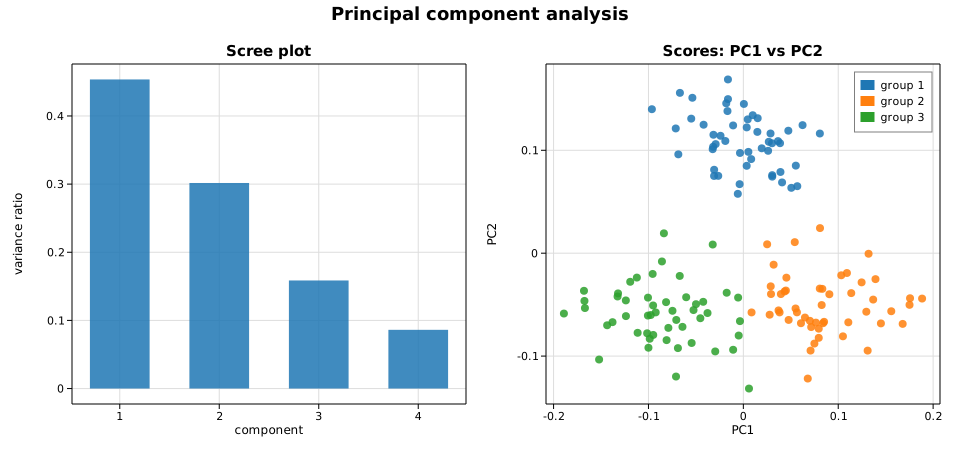
This example generates three clusters in a 4-dimensional feature space, fits PCA on the standardized columns, and produces two classic diagnostics: a scree plot of the per-component variance ratio and a scores scatter of the first two principal components.
Code
#![allow(unused)]
fn main() {
use ndarray::Array2;
use solow_multivariate::Pca;

// Three latent groups in 4-D; 50 points each.
let matrix = Array2::from_shape_vec((n, 4), data).unwrap();

// Fit on standardized columns.
let res = Pca::new(matrix).standardize(true).fit().unwrap();

// Results expose eigenvals, explained_variance_ratio, loadings, and scores.
for i in 0..res.ncomp {
    println!("comp {}: ratio = {:.4}", i + 1, res.explained_variance_ratio[i]);
}
// res.scores is nobs x ncomp; columns 0 and 1 are PC1 and PC2.
}
Printed summary
PCA on 150 observations x 4 variables
  comp    eigenvalue       var ratio      cumulative
     1      272.1529          0.4536          0.4536
     2      180.9883          0.3016          0.7552
     3       95.1618          0.1586          0.9138
     4       51.6970          0.0862          1.0000
The first two components together capture about 76% of the total variance — and, as the scores plot shows, they are exactly the directions that separate the three groups.
Plot
Left: the scree plot (variance ratio per component). Right: the PC1/PC2 scores, colored by the true group label — the three clusters are cleanly separated in the leading two-component subspace.