Generalized additive models (smooth fit)
A generalized additive model replaces the linear predictor of a GLM with a sum
of smooth functions of the covariates. This example fits a Gaussian GAM with a
single penalized B-spline smooth term to a noisy nonlinear signal using
GlmGam. The smooth is estimated by penalized
iteratively reweighted least squares (P-IRLS) at a fixed smoothing parameter
alpha; the curvature penalty trades wiggliness against fit, and the resulting
effective degrees of freedom measure how flexible the fitted curve is.
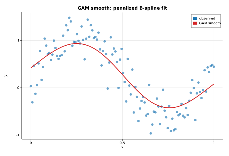
The true signal is f(x) = sin(2πx) + 0.5x corrupted by Gaussian noise. We fit
a cubic (degree = 3) B-spline basis with df = 12 (which yields 11 basis
columns once the constant column is dropped) and a light penalty, then overlay
the fitted smooth on the scatter.
Code
#![allow(unused)]
fn main() {
use ndarray::Array1;
use solow_gam::GlmGam;
use solow_glm::Family;
use solow_viz::{Color, Figure, LegendLoc, LineStyle, Marker};

// Example data: x in [0, 1];  f(x) = sin(2 pi x) + 0.5 x;  y = f(x) + N(0, 0.25^2)
let n = 120usize;
let sigma = 0.25;
let x = Array1::linspace(0.0, 1.0, n);
let signal = x.mapv(|xi| (std::f64::consts::TAU * xi).sin() + 0.5 * xi);
// y is signal plus deterministic pseudo-random Gaussian noise.

// Fit a penalized B-spline GAM (Gaussian, canonical identity link).
let df = 12usize;
let degree = 3usize;
let alpha = 0.01;
let res = GlmGam::new(y.clone(), &x, df, degree, alpha, Family::Gaussian)
    .unwrap()
    .fit()
    .unwrap();

println!("intercept         : {:.6}", res.intercept());
println!("edf (total)       : {:.6}", res.edf_total);
println!("scale (sigma^2)   : {:.6}", res.scale);
println!("deviance          : {:.6}", res.deviance);
}
The fitted means (res.fittedvalues) are evaluated at the observations, so the
smooth curve is drawn directly through x:
#![allow(unused)]
fn main() {
let x_vec: Vec<f64> = x.to_vec();
let fit_vec: Vec<f64> = res.fittedvalues.to_vec();

let mut fig = Figure::new(760, 520);
let ax = fig.axes();
ax.set_title("GAM smooth: penalized B-spline fit")
    .set_xlabel("x").set_ylabel("y").set_grid(true);
ax.scatter_full(&x_vec, &y_vec, Color::cycle(0), 4.0, Marker::Circle, 0.65, Some("observed"));
ax.line(&x_vec, &fit_vec, Color::RED, 2.5, LineStyle::Solid, Marker::None, 1.0, Some("GAM smooth"));
ax.legend(LegendLoc::UpperRight);
fig.save_svg("gam_smooth.svg").unwrap();
}
Printed results
Generalized additive model (penalized B-spline smooth)
------------------------------------------------------
family            : Gaussian (identity link)
basis             : 11 cubic B-spline columns (df=12)
smoothing alpha   : 0.01
converged         : true (in 2 iters)
intercept         : 0.419307
edf (total)       : 4.095559
df_resid          : 115.904441
scale (sigma^2)   : 0.098754
deviance          : 11.446068
penalized deviance: 17.048607
resid. std (est)  : 0.314252   (true sigma = 0.25)
The fit uses about 4.1 effective degrees of freedom — far fewer than the 12
nominal basis dimensions — capturing the sinusoidal shape plus the gentle linear
trend without chasing the noise. The estimated residual standard deviation
(0.314) is close to the true 0.25, the small excess reflecting the smooth's
slight bias where the penalty rounds off the peaks.
Plot