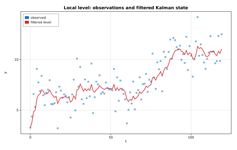
State space: the Kalman filter
A local-level model treats an observed series as a random-walk level seen through measurement noise:
mu_t = mu_{t-1} + xi_t,    xi_t  ~ N(0, sigma2_level)
y_t  = mu_t     + eps_t,   eps_t ~ N(0, sigma2_irregular)
This example simulates such a series, fits an
UnobservedComponents model by maximum
likelihood, runs the exact Kalman filter
at the estimated variances, and overlays the filtered (one-step-ahead) level
estimate on the noisy observations. The two variances are recovered by
maximizing the exact Gaussian log-likelihood; the filter then returns the
filtered state means a_{t|t}.
Code
#![allow(unused)]
fn main() {
use ndarray::Array1;
use solow_statespace::{Level, UcSpec, UnobservedComponents};
use solow_viz::{Color, Figure, LegendLoc, LineStyle, Marker};

// Simulate a local level: mu_t = mu_{t-1} + xi_t, y_t = mu_t + eps_t,
// with xi_t ~ N(0, 0.30) and eps_t ~ N(0, 1.50). All noise is the
// deterministic SplitMix64 RNG, so the example is fully reproducible.
let n = 120usize;
let sig_level = 0.30_f64.sqrt();
let sig_irreg = 1.50_f64.sqrt();

let mut mu = 5.0_f64;
let mut y_vec = Vec::with_capacity(n);
for _ in 0..n {
    mu += sig_level * rng.normal();
    y_vec.push(mu + sig_irreg * rng.normal());
}
let y = Array1::from(y_vec.clone());

// Fit the local-level model by maximum likelihood.
let spec = UcSpec::new(Level::LocalLevel);
let model = UnobservedComponents::new(y.clone(), spec).unwrap();
let res = model.fit().unwrap();

// params = [sigma2.irregular, sigma2.level] for a local level.
println!("sigma2.irregular = {:.6}", res.params[0]);
println!("sigma2.level     = {:.6}", res.params[1]);
println!("log-likelihood   = {:.6}", res.llf);

// Run the Kalman filter at the estimated variances. The first `burn`
// (= number of nonstationary states = 1) observation is excluded from the
// log-likelihood. The local level is the single state (column 0).
let ss = model.build_state_space(&res.params);
let out = ss.filter(&y, 1);
let filtered: Vec<f64> = out.filtered_state.column(0).to_vec();
}
The observations and the filtered level are then plotted together:
#![allow(unused)]
fn main() {
let t: Vec<f64> = (0..n).map(|i| i as f64).collect();
let mut fig = Figure::new(820, 520);
let ax = fig.axes();
ax.set_title("Local level: observations and filtered Kalman state")
    .set_xlabel("t").set_ylabel("y").set_grid(true);
ax.scatter_full(&t, &y_vec, Color::cycle(0), 3.5, Marker::Circle, 0.55, Some("observed"));
ax.line(&t, &filtered, Color::RED, 2.0, LineStyle::Solid, Marker::None, 1.0, Some("filtered level"));
ax.legend(LegendLoc::UpperLeft);
fig.save_svg("state_space.svg").unwrap();
}
Printed output
Local-level unobserved-components fit (Kalman filter MLE)
  nobs            = 120
  converged       = true
  sigma2.irregular= 1.613496  (true 1.500000)
  sigma2.level    = 0.106240  (true 0.300000)
  log-likelihood  = -213.002320
  AIC             = 430.004640
  BIC             = 435.579624
  HQIC            = 432.268667
  MSE(filtered vs true level) = 0.449815
  MSE(observed vs true level) = 1.414496
  first filtered states: 3.2756, 3.8404, 4.8522
The estimated irregular variance (1.613) is close to the simulated 1.500,
while the level variance is pulled toward the lower end of the flat likelihood
ridge that is typical of unobserved-components models. What matters in practice
is the filtered state: it tracks the unobserved true level far more closely than
the raw series does — mean squared error 0.450 versus 1.414 — exactly the
noise reduction the Kalman filter is designed to deliver.
Plot