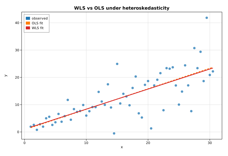
Weighted & generalized least squares (WLS / GLS)
When the error variance is not constant across observations
(heteroskedasticity), ordinary least squares stays unbiased but is no longer
efficient, and its standard errors are wrong. Weighted least squares fixes
this by weighting each observation by the inverse of its error variance.
Generalized least squares is the general form: supply the full error
covariance matrix Σ. With a diagonal Σ, GLS reduces exactly to WLS.
This example builds data whose noise standard deviation grows with x, then
fits OLS, WLS, and GLS for comparison.
Code
#![allow(unused)]
fn main() {
use ndarray::{Array1, Array2};
use solow_core::tools::{add_constant, HasConstant};
use solow_regression::LinearModel;

// Heteroskedastic data: the noise sd scales with x, so later points are noisier.
let n = 60usize;
let x_raw: Vec<f64> = (0..n).map(|i| 1.0 + i as f64 * 0.5).collect();
let sd: Vec<f64> = x_raw.iter().map(|&xi| 0.35 * xi).collect();
// y_vec = 1 + 0.8 x + sd * noise

let x = Array2::from_shape_vec((n, 1), x_raw.clone()).unwrap();
let y = Array1::from(y_vec.clone());
let design = add_constant(&x, true, HasConstant::Add).unwrap();

// Weights proportional to 1 / variance; Sigma is the diagonal variance matrix.
let weights = Array1::from(sd.iter().map(|&s| 1.0 / (s * s)).collect::<Vec<_>>());
let mut sigma = Array2::<f64>::zeros((n, n));
for i in 0..n { sigma[[i, i]] = sd[i] * sd[i]; }

let ols = LinearModel::ols(y.clone(), design.clone()).unwrap().fit().unwrap();
let wls = LinearModel::wls(y.clone(), design.clone(), weights).unwrap().fit().unwrap();
let gls = LinearModel::gls(y.clone(), design.clone(), &sigma).unwrap().fit().unwrap();
}
Printed summary
OLS treats every point as equally informative:
                            OLS Regression Results
==============================================================================
Dep. Variable:                       y   R-squared:                     0.565
Model:                             OLS   Adj. R-squared:                0.558
No. Observations:                    60   F-statistic:                   75.47
==============================================================================
                   coef    std err         t     P>|t|      [0.025      0.975]
------------------------------------------------------------------------------
const            0.7950      1.555     0.511     0.611      -2.317       3.907
x                0.7514      0.086     8.687     0.000       0.578       0.925
==============================================================================
WLS downweights the noisy high-x points, tightening the standard errors:
                            WLS Regression Results
==============================================================================
Dep. Variable:                       y   R-squared:                     0.743
Model:                             WLS   Adj. R-squared:                0.739
No. Observations:                    60   F-statistic:                   167.8
==============================================================================
                   coef    std err         t     P>|t|      [0.025      0.975]
------------------------------------------------------------------------------
const            1.0254      0.277     3.703     0.000       0.471       1.580
x                0.7345      0.057    12.955     0.000       0.621       0.848
==============================================================================
The WLS intercept standard error drops from 1.555 to 0.277. And GLS with a
diagonal Σ reproduces the WLS coefficients to the bit:
GLS with diagonal Sigma reproduces the WLS coefficients exactly:
  WLS params = [1.025374, 0.734467]
  GLS params = [1.025374, 0.734467]
Plot
The dashed OLS line is tilted by the high-variance points; the solid WLS line tracks the underlying relationship more faithfully.